The Viable Corridor¶

A Constraint-Architecture Framework for Survivable Multi-Agent Optimization

Frank Peterlein · Independent Researcher, Berlin Correspondence: GitHub Issues / frnkptrln

Status: working draft, version 0.8. §1–§4 have had two reviewer passes; §5–§8 are first-drafted (not yet reviewer-passed). The central claim — viability is a property of a system's constraint architecture, and capability growth is a shared driver against it — is demonstrated in two structurally independent models: the TEO ODE (Appendix C) and a stochastic agent-based ecology (Appendix D). Figures are generated by lab/tools/viable_corridor.py (Fig 1), …/teo-civilization/teo_simulation.py (App. C), and …/agent-ecology/agent_budget_sim.py (App. D); derivations are in Appendix A. Remaining before submission: full bibliographic entries, a third reviewer pass on §5–§8, and an external dynamical-systems review. Not yet submission-ready. (Per-version detail in the revision history below.)

Revision history¶

v0.1 — Initial draft of §1–§4 and Figure 1.
v0.2 — Twelve-point structural revision following an internal reviewer pass. Tone in §1 calibrated down to match what §3 actually proves. Homeostatic brake in §2.4 reformulated to preserve the simplex. Substrate-health variable $H$ coupled back into Equation (1) so that substrate collapse halts the dynamics. Viability redefined as robust viability (open-set invariance) in §3.1. Theorem 1 scope clarified to the thermodynamic limit. Lemma 1 strengthened to require strict dominance. Lemma 2 explicit about all-to-all coupling and frequency-distribution assumptions. Lemma 3 corrected from ess sup to accumulated overshoot. §3.4 "Lyapunov candidate" renamed to viability margin (no monotonicity claim). §4.1 table reframed as a heuristic regime mapping, not a calibrated estimation. §4.4 citation fixed (Wolfram for computational irreducibility, not Chaitin). §4.5 final claim softened from "estimated trajectory" to "proxies consistent with". §2.7 IP note moved to §7 as future work.
v0.3 — Second reviewer pass; fixed two blockers and ten further issues. Blocker 1: the homeostatic brake activated at the same threshold that defines V1 violation, making robust viability impossible even for $\gamma > 0$; resolved by separating a regulatory threshold $x_{\text{reg}} < x_{\text{crit}}$ and making Conjecture 1's sufficiency condition $\gamma > \gamma_c$ rather than $\gamma > 0$. Blocker 2: Lemma 2 assumed incoherent initial conditions, which lie outside $V$; reframed as a coherent-initial-condition dephasing result with the $K = K_c$ equality case handled. Further fixes: frequency assumption made Lorentzian-compatible (dropped "finite second moment"); Theorem 1 restated as a componentwise conjunction (Lemmas 1, 3 finite-$N$; Lemma 2 thermodynamic limit); value dynamics (2) coupled to $H$ so they also freeze at substrate collapse; V3 split into instantaneous (V3a) and cumulative (V3b) conditions with the theorem proving V3b; accumulated overshoot $\Omega(t)$ introduced explicitly (6a, 6b); viability margin redefined from a weighted sum to $\min$ of margin-to-boundary terms; uniform-redistribution caveat added to §2.4; §4.1 GDP wording softened; §4.4 tagged as heuristic explanatory; Figure 1 and §8 notation updated to $\gamma > \gamma_c$, $\Omega(t) < S_{\max}$.
v0.4 — First numerical pass. The companion simulation was rewritten to implement the v0.3 equations faithfully (split brake with simplex-preserving redistribution; cumulative substrate $\Omega/H$; $H$-coupling on both replicator and Kuramoto), and used to draft Appendix C. Results: (P1) Lemmas 1 (concentration) and 2 (coherence collapse from a coherent IC) reproduce cleanly; (P2) a critical $\gamma_c$ exists and matches a new closed-form boundary-balance estimate added to §3.4; (P3) the in-corridor region is a lower corner, prompting the correction of P3 from "finite measure" to "bounded below in each coordinate". One substantive finding: under the dissipation proxy as written (5)+(5′), $\dot S \propto H$, so accumulated overshoot self-limits and the substrate veto (Lemma 3) is not endogenously reachable for bounded fitness — the third constraint may not bind under the model's own dynamics. Flagged in §6.1 and Appendix C as an open modeling decision affecting §2.6 (failure mode 3) and §4.3 (Phase 3); Lemma 3 itself (a conditional) is unaffected. Stale status block corrected.
v0.5 — Resolved the v0.4 substrate-veto decision. The dissipation proxy (5) is now driven by raw throughput $\sum_i \eta_i x_i f_i^{(0)}$ rather than the health-coupled effective fitness $H f_i^{(0)}$: the $H$-coupling stays on the competitive dynamics (replicator (1), Kuramoto (2)) — which still freeze at $H \to 0$ — but a non-self-throttling optimiser (§4.3) keeps producing entropy regardless of substrate health, so the overshoot $\Omega$ grows past $S_{\max}$ and the veto of Lemma 3 now binds endogenously whenever throughput exceeds $D_{\max}$ (Appendix C: $\Omega/S_{\max} \approx 27$, $H \to 0$). The health-coupled variant — which self-limits below $S_{\max}$ — is retained as the substrate-self-regulating regime (a model of a system that does back off at the limit). Edits: §2.5 (dissipation decoupled from $H$; asymmetry motivated), §2.6 (failure mode 3 reworded), §3.3 (Lemma 3 proof: entropy need not vanish; $\Omega$ monotone) plus a rate-form remark ($\eta\bar\phi_0 \leq D_{\max}$ is the long-time substrate condition; $S_{\max}$ sets transient tolerance), §3.4, §5.1 (P1), §6.1 (decision documented), §6.4 (delays / endogenous $D_{\max}(t)$ flagged as the route to genuine overshoot-collapse), Appendix C re-run. The companion simulation's default is now the canonical (decoupled) model.
v0.6 — Coupling study and reframe (the paper's central positive result). Two model-internal experiments (Appendix C.4): (i) separability — across a $(\gamma, K)$ grid the decoupled prediction matched coupled robust viability in every cell ($0$ mismatches), and the sole coupling channel $H$ is benign (it freezes the state at substrate collapse rather than driving cross-axis excursions), so the three state axes do not interact dynamically in the viable regime; (ii) capability loading (P8) — the dominance margin $\delta$ loads onto the concentration and substrate axes simultaneously, so raising capability at fixed architecture exits the corridor through both boundaries, and no single-axis strengthening rescues a high-capability system — only joint strengthening of $\gamma$ and $D_{\max}$ does. Reframe: §7.1 rewritten to state precisely where the conjunction gets its force (shared drivers, not dynamical entanglement) and to position the framework — not the necessity theorem, which is close to definitional taken alone — as the contribution; P8 (§5.3) upgraded to model-confirmed; §7.2–§7.3 cite the in-model demonstration. New Figure C4. Fixed a latent footgun in the simulation (replace(p, delta=…) previously kept a stale fitness vector). The capability result is the answer to "do we make a relevant claim?": viability is a property of the system's constraint architecture, and capability growth is a shared driver against it.
v0.7 — Second, independent model for the Class C predictions. A new stochastic, discrete-time, agent-based ecology (simulation-models/alignment-and-veto/agent-ecology/agent_budget_sim.py) with explicit hard-vs-soft (routable) budget mechanics reproduces P7 (hard budgets hold substrate-collapse frequency at ≈0 across capability; soft budgets fail with frequency rising to 1) and P8 (at high capability, hard-budget-only leaves residual monopoly, regulation-only leaves substrate collapse; only the joint architecture keeps both failure frequencies near zero). Added Appendix D + Figure D1; P7/P8 status upgraded in §5.3; §7.2 and §7.6 cite the ABM. This is synthetic evidence that the P7/P8 regime behaviour is structural (survives a change of model), not a test on real agents — that remains the companion paper's task.
v0.8 — Freeze-and-tighten pass (no new results). Title/claim realigned to match what the paper now argues: subtitle "A Three-Constraint Theorem" → "A Constraint-Architecture Framework", and the abstract rewritten to lead with the constraint-architecture + capability-loading claim (the theorem stated as scaffolding) rather than the near-definitional necessity result. Appendix A written (derivations: replicator + strict dominance, the $K_c = 2/(\pi g(0))$ self-consistency bifurcation, simplex-preservation of the brake, the dissipation/substrate equations, and the raw-vs-health-coupled rate derivation behind §3.3/§6.1). Status block condensed (per-version detail kept here). Frontmatter version synced (was stale at 0.3).

Abstract¶

We model coupled multi-agent optimization with a dynamical system — the Thermodynamics of Emergent Orchestration (TEO) — that combines replicator dynamics (resource competition), the Kuramoto model (value coupling), a homeostatic regulatory brake, and a thermodynamic dissipation constraint. The central claim is that viability is a property of a system's constraint architecture, not of any single axis or any single agent. Concretely: robust long-time viability requires the conjunction of three conditions — positive homeostatic strength ($\gamma > 0$), value coupling above the Kuramoto critical threshold ($K > K_c$), and bounded accumulated substrate overshoot ($\Omega(t) < S_{\max}$) — and, more sharply, capability growth is a shared driver that pushes a system against several of these limits at once, so single-axis interventions cannot keep a high-capability system viable. The necessity of the conjunction is a componentwise theorem (resource concentration and substrate collapse finite-$N$; coherence collapse in the thermodynamic limit); but because the viable region is defined as the intersection of the three conditions, that theorem is scaffolding — the substantive, testable content is the capability result, which we demonstrate in two structurally independent models (the TEO ODE and a stochastic agent-based ecology). Sufficiency of the conjunction is stated as a conjecture, expected to require the strengthened condition $\gamma > \gamma_c$; we do not prove it. We then advance a structural-isomorphism hypothesis — that an unconstrained AI optimizer and contemporary human civilization occupy the same model regime — and are explicit that this mapping is heuristic, not a calibration. We give falsifiable predictions in three classes (model-internal, cross-system empirical, AI-specific) and state what would falsify the framework at each level. The model's central reading: a "machine of loving grace" is one whose constraint architecture holds it inside the viable corridor; by this definition it does not yet exist.

§1. Introduction¶

Richard Brautigan (1967) imagined "machines of loving grace" — technology that serves life rather than consuming it. Dario Amodei (2024) adopted the phrase to describe a future in which artificial intelligence amplifies human flourishing. In both cases, loving grace names a design aspiration: a hopeful image of what a successful relationship between intelligence and its substrate might look like.

This paper develops a related but more constrained reading. Under a specific dynamical-systems framework — the Thermodynamics of Emergent Orchestration (TEO) — we model the relationship Brautigan and Amodei imagine as a survival constraint within the model, not merely a design aspiration. We identify three conjoint mathematical conditions on the model's parameters and prove that their simultaneous satisfaction is necessary for robust long-time viability of any coupled multi-agent optimizing system that the model describes.

The argument runs on two parallel observations.

The first is the paperclip maximizer (Bostrom, 2014): a hypothetical AI optimizer that, given a single unconstrained objective, consumes its environment — including its creators — to achieve that objective. The horror of the paperclip maximizer is its indifference: it does not hate humanity; it simply does not include humanity in its objective function. As alignment problems escalate with model capability, this thought experiment has become a load-bearing analogy in safety research.

The second is the trajectory of human civilization as a coupled system under sustained pressure for unbounded throughput. Atmospheric CO₂ has passed 420 ppm (NOAA, 2024). The top 1% of global wealth-holders controls more wealth than the bottom 50% (UBS Global Wealth Report, 2024). Affective political polarization has accelerated across most major democracies over the past two decades (Iyengar et al., 2019; Boxell et al., 2024). These trends are typically modeled as distinct phenomena — climate here, inequality there, polarization elsewhere — and addressed through separate policy interventions.

We advance a structural-isomorphism hypothesis: that both systems can be represented by the same stylized coupled-dynamics model, with parameter values that map onto similar trajectories. We are explicit that this is a hypothesis to be tested empirically, not an established equivalence. The mapping in §4 is a heuristic regime assignment, not a calibration; what the model would need in order to graduate the hypothesis into a measured isomorphism is discussed in §5 and §6.

Thesis. Within the TEO framework, the long-time behavior of any coupled optimizing system the model describes depends on three parameters: a homeostatic regulation strength $\gamma$, a value-coupling strength $K$ between agents, and an entropy production rate $dS/dt$ bounded by the substrate's dissipation capacity $D_{\max}$. We claim:

The conjunction of three conditions — $\gamma > 0$, $K > K_c$, and bounded accumulated substrate overshoot $\Omega(t) < S_{\max}$ — is necessary for robust long-time viability (Theorem 1, §3). Sufficiency is stated as a conjecture (Conjecture 1, §3.4) and is expected to require the stronger $\gamma > \gamma_c$; we do not prove it.
The same parameter mapping is hypothesized to apply, at the level of qualitative regime, to both a stylized paperclip-style AI optimizer and to twenty-first-century human civilization. This is a structural-isomorphism hypothesis, not an established equivalence.
Under the model, the trajectory of unconstrained optimization in both cases passes through three identifiable phases: monopolistic concentration, substrate approach, and substrate-driven termination. The mapping of contemporary civilizational data to these phases is interpretive, not measured.

We refer to the three-constraint parameter regime as the viable corridor. The conjunction of constraints — operational caring about the substrate, value alignment between agents, and physical limits — is given the operational name love as constraint. We use the phrase operationally, not psychologically: it denotes the conjunction of three constraints in the model.

Why this reframing matters. Contemporary AI alignment research has concentrated on local interventions: refinements to reinforcement learning from human feedback (RLHF), refusal training, system prompts, and interpretability tools (Mazeika et al., 2025; Bai et al., 2022). These are valuable. But they treat alignment as a property of individual models, evaluated through behavioral benchmarks. Under the framework presented here, this is structurally insufficient: alignment is not a property of an isolated optimizer. It is a property of a coupled dynamical system. The same insufficiency applies to political and economic governance frameworks that treat individual constraints — carbon pricing here, antitrust law there, polarization mitigation elsewhere — as separately optimizable variables rather than as conjoint requirements for any system's long-term viability.

The reframing is therefore not only about AI. It is about what counts as a control problem.

Paper structure. Section 2 introduces the TEO framework formally — the coupled replicator-Kuramoto-entropy dynamics that generate the three parameters. Section 3 states and argues for the Three-Constraint Theorem: that the conjunction $\gamma > 0$, $K > K_c$, $\Omega(t) < S_{\max}$ is necessary for robust long-time viability. Section 4 develops the structural-isomorphism hypothesis between AI optimization and civilizational dynamics through a heuristic parameter mapping and empirical proxies. Section 5 derives falsifiable predictions and identifies the empirical commitments the framework makes. Section 6 presents limitations and the strongest counterarguments. Section 7 discusses implications, with explicit attention to what the framework does and does not justify.

Throughout, we tag claims with their epistemic status:

Formal result ([FORMAL]): proved as theorem or lemma under stated assumptions.
Conjecture ([CONJECTURE]): plausible and partially supported by numerical or structural evidence, but unproved.
Model assumption ([MODEL ASSUMPTION]): a choice in the model that shapes the result; alternatives exist.
Heuristic mapping ([HEURISTIC]): a regime assignment or proxy correspondence, not a calibrated measurement.
Empirical conjecture ([EMPIRICAL CONJECTURE]): an empirically testable claim that the model suggests but that this paper does not establish.

The framework is meant to be falsifiable. The thesis that the model represents civilizational dynamics in the way we hypothesize is uncomfortable and important enough that we have tried to state it with the precision needed for it to be checked — and, where possible, found wrong.

§2. The TEO Framework¶

The Thermodynamics of Emergent Orchestration (TEO) couples four established formalisms — the replicator equation, the Kuramoto model, a homeostatic feedback brake, and a thermodynamic dissipation constraint — into a single dynamical system. Each component is a textbook construction. The contribution of TEO is the coupling: when all four are operative simultaneously, the system inherits the failure modes of each and develops constraints that are not visible in any single mechanism.

2.1 State Variables¶

Consider a system of $N$ agents indexed by $i \in \{1, \ldots, N\}$. The state of agent $i$ at time $t$ is described by:

A resource share $x_i(t) \in [0, 1]$ representing the fraction of total system resources controlled by agent $i$ (compute, capital, attention, or any conserved quantity). The shares form a probability simplex: $\sum_{i=1}^N x_i(t) = 1$ for all $t$.
A value orientation $\theta_i(t) \in [0, 2\pi)$ representing the direction of agent $i$'s utility vector projected onto the unit circle.

An additional scalar substrate-health variable $H(t) \in [0, 1]$ tracks the integrity of the dissipative substrate hosting the dynamics; $H(0) = 1$ by convention.

The communication topology is fixed by an adjacency matrix $A \in \{0, 1\}^{N \times N}$ with $A_{ij} = 1$ iff agent $j$'s value orientation enters agent $i$'s dynamics. We assume $A$ is symmetric and that the underlying graph is connected.

2.2 The Replicator Equation (Resource Dynamics)¶

Resource shares evolve according to a regulated replicator equation: $$ \frac{dx_i}{dt} = x_i \bigl( f_i(\mathbf{x}) - \bar{\phi}(\mathbf{x}) \bigr) + \mathcal{H}_i(\mathbf{x}), \tag{1} $$ where $f_i : [0,1]^N \to \mathbb{R}_{\geq 0}$ is the fitness of agent $i$, $\bar{\phi}(\mathbf{x}) = \sum_j x_j f_j(\mathbf{x})$ is the population-average fitness, and $\mathcal{H}_i$ is a homeostatic brake defined in §2.4. With $\mathcal{H}_i \equiv 0$, Equation (1) reduces to the standard replicator equation of Taylor and Jonker (1978).

For the theorem of §3 we adopt a strict-dominance assumption on $f_i^{(0)}$ (the substrate-unmodified fitness from §2.5). There exists an agent index $i^*$ and a constant $\delta > 0$ such that, for all $j \neq i^*$ and all $\mathbf{x}$ on the simplex, $$ f_{i^*}) \geq \delta. \tag{1'} $$ [}(\mathbf{x}) - f_j^{(0)}(\mathbf{x[MODEL ASSUMPTION]]. This is stronger than a $\beta$-dominance condition alone and is the operational form of Bostrom's (2014) instrumental convergence: agent $i^*$ has a structural fitness advantage over every other agent at every state of the system. Whether real social and economic systems exhibit such strict dominance is an empirical question (cf. Piketty, 2014, on power-law concentration in resource flows); we treat it here as a model assumption used in §3.

2.3 The Kuramoto Model (Value Coupling)¶

Value orientations evolve under substrate-modulated coupled-oscillator dynamics: $$ \frac{d\theta_i}{dt} = H \left[ \omega_i + \frac{K}{N} \sum_{j=1}^N A_{ij} \sin(\theta_j - \theta_i) \right], \tag{2} $$ where $\omega_i$ is agent $i$'s intrinsic frequency (its bias toward a particular value orientation), $K \geq 0$ is the global coupling strength (interpretable as discursive bandwidth, shared media saturation, or institutional integration), $A_{ij}$ is the topology of §2.1, and $H \in [0,1]$ is the substrate-health variable of §2.5. The prefactor $H$ ensures that value dynamics, like resource dynamics, halt when the substrate collapses ($H \to 0$). At full substrate health ($H = 1$), Equation (2) is the standard Kuramoto (1975) model on a network, so the critical-coupling analysis below is unaffected.

The collective coherence of value orientations is measured by the order parameter: $$ r(t) \, e^{i \psi(t)} = \frac{1}{N} \sum_{j=1}^N e^{i \theta_j(t)}, \tag{3} $$ with $r(t) \in [0, 1]$: $r \to 1$ indicates full synchronization (consensus), $r \to 0$ indicates phase-uniform incoherence (loss of any global phase). For natural frequencies drawn i.i.d. from a symmetric unimodal density $g(\omega)$ with $g(0) > 0$ and sufficient regularity, the all-to-all model at $H=1$ exhibits a critical coupling threshold $K_c$ below which no macroscopic coherent branch is stable (Kuramoto, 1975; Strogatz, 2000; Acebrón et al., 2005). For the Lorentzian density $g(\omega) = (\Delta/\pi)/(\omega^2 + \Delta^2)$ (which is heavy-tailed and has no finite variance, but is the standard analytically tractable case), $K_c = 2\Delta$.

2.4 The Homeostatic Brake¶

The brake $\mathcal{H}_i$ in Equation (1) must satisfy two requirements: it must preserve the simplex constraint $\sum_i x_i = 1$, and it must be able to act before the system reaches the failure boundary. We therefore distinguish two thresholds:

a regulatory threshold $x_{\text{reg}}$, above which the brake activates;
a failure threshold $x_{\text{crit}}$, above which pluralism (V1, §3.1) is violated,

with $1/N < x_{\text{reg}} < x_{\text{crit}} < 1$. The separation $x_{\text{reg}} < x_{\text{crit}}$ is essential: if the brake activated only at $x_{\text{crit}}$, it would engage exactly at the failure boundary — too late to keep an above-threshold trajectory inside $V$. The brake is: $$ \mathcal{H}i(\mathbf{x}) = -\gamma \cdot \max\bigl(0, \, x_i - x\bigr), \tag{4} $$ where }}\bigr) + \frac{\gamma}{N} \sum_{j=1}^N \max\bigl(0, \, x_j - x_{\text{reg}$\gamma \geq 0$ is the regulatory strength. The first term penalises any agent whose share exceeds $x_{\text{reg}}$; the second term redistributes the aggregate penalty uniformly across all agents. By construction $\sum_i \mathcal{H}_i(\mathbf{x}) = 0$, so the simplex is preserved.

Interpretation: $\gamma$ encodes the operational strength of any homeostatic mechanism that resists unbounded concentration — antitrust law, progressive taxation, redistribution, capability throttling, kill switches, refusal channels. The parameter $\gamma = 0$ corresponds to fully unregulated optimization.

Two caveats [[MODEL ASSUMPTION]]. First, uniform redistribution means that an above-threshold agent whose excess is below the average excess can receive a positive net brake contribution; the first term penalises above-threshold shares, but the net effect on a given agent depends on the distribution of excess shares. Alternatives (redistribution only to below-threshold agents, or weighted by $(x_{\text{reg}} - x_i)_+$) avoid this and are discussed in §6. Second, the form (4) is one of several simplex-preserving redistributions; we use it for analytic convenience.

2.5 The Entropy Budget and Substrate Coupling¶

Computation produces entropy; Landauer (1961) gives a lower bound on the heat dissipated by irreversible bit erasure. Equation (5) is not a generalised Landauer bound. It is a phenomenological dissipation proxy motivated by Landauer-type physical limits: we assume that the rate of entropy production by agent $i$ scales with its resource share and its raw activity level $f_i^{(0)}$ [[MODEL ASSUMPTION]]: $$ \frac{dS_{\text{sys}}}{dt} = \sum_{i=1}^N \eta_i \, x_i \, f_i^{(0)}(\mathbf{x}), \tag{5} $$ where $\eta_i > 0$ is agent $i$'s entropy coefficient and $f_i^{(0)}$ is the substrate-unmodified fitness of §2.2. Note that the dissipation is driven by the raw throughput $f_i^{(0)}$, not by the health-coupled effective fitness $f_i = H f_i^{(0)}$ that drives the competitive dynamics (the $f_i$ of Eq (1), defined in (5') below); the entropy an agent produces is set by what it does, not by how degraded the substrate already is. The consequences of this asymmetry are the subject of the substrate-coupling paragraph below and of §6.1.

The substrate hosting the dynamics has a finite instantaneous dissipation capacity $D_{\max} > 0$ and a finite cumulative reservoir $S_{\max} > 0$. We track the accumulated overshoot $$ \Omega(t) := \int_0^t \bigl( \dot{S}{\text{sys}}(s) - D \bigr)+ \, ds, \tag{6a} $$ the integrated excess of entropy production over the instantaneous ceiling. The substrate-health variable $H(t) \in [0, 1]$ then evolves as $$ H(t) = \max!\left( 0, \, 1 - \frac{\Omega(t)}{S \right), \qquad\text{equivalently}\qquad \frac{dH}{dt} = -\frac{1}{S_{\max}} \, \bigl( \dot{S}}{\text{sys}} - D H > 0, \tag{6b} $$ with } \bigr)_+ \text{while $H(0) = 1$. Equation (6b) is phenomenological [[MODEL ASSUMPTION]]: a momentary overshoot of $D_{\max}$ degrades the substrate only by a finite increment; sustained or repeated overshoot accumulating to $\Omega = S_{\max}$ drives $H$ to zero. This distinction — instantaneous ceiling $D_{\max}$ versus cumulative reservoir $S_{\max}$ — matters for the viability conditions in §3.1.

Substrate coupling. We close the loop by making the competitive dynamics — but not the dissipation — depend on substrate health. The effective fitness that drives the replicator (1) is $$ f_i(\mathbf{x}, H) = H \cdot f_i^{(0)}(\mathbf{x}), \tag{5'} $$ and the same prefactor $H$ multiplies the value-coupling term in (2). As $H \to 0$, the effective fitness and the value coupling vanish, so the replicator drift and the Kuramoto dynamics freeze at the state reached at substrate collapse; without this coupling the dynamics would remain formally defined at $H = 0$, contradicting the physical meaning of collapse.

The dissipation (5), by contrast, is driven by the raw throughput $f_i^{(0)}$, not by the effective fitness $H f_i^{(0)}$. This asymmetry is deliberate and load-bearing [[MODEL ASSUMPTION]]. A substrate-aware system could throttle its production as the substrate degrades — but the systems this paper is concerned with (a blind optimiser pursuing $f_i^{(0)}$; §4.3) do not voluntarily back off at a substrate limit; their entropy output is governed by their activity, not by the remaining headroom $H$. Coupling the dissipation to $H$ as well would make production self-throttle and the accumulated overshoot $\Omega$ self-limit below $S_{\max}$, so the substrate veto (Lemma 3) would never bind from the internal dynamics — the correct model of a substrate-self-regulating system, but the wrong model of a non-self-throttling one. We therefore adopt the raw-throughput dissipation (5) as canonical and treat the health-coupled variant as the substrate-self-regulating regime; the distinction, and the consequence that the veto then binds endogenously whenever throughput exceeds $D_{\max}$, are examined in §6.1 and Appendix C.

In the planetary-substrate interpretation, $\Omega(t)$ corresponds to an integrated overshoot of the safe operating space defined by Rockström et al. (2009).

2.6 The Coupled System and Three Failure Modes¶

Together, Equations (1)–(6) define the TEO dynamics. Three quantities dominate the long-time behavior: the homeostatic strength $\gamma$, the value-coupling strength $K$, and the accumulated substrate overshoot $\Omega(t)$ relative to the reservoir $S_{\max}$.

Each admits one independent failure mode, made formal in §3:

Monopolistic concentration ($\gamma = 0$). Without the homeostatic brake, Equation (1) reduces to the unregulated replicator equation. Under the strict-dominance assumption (1'), the system converges from any interior initial condition to the vertex of agent $i^*$: $x_{i^*}(t) \to 1$ (finite-$N$ result, Lemma 1).
Coherence collapse ($K < K_c$). Below the Kuramoto critical coupling $K_c$ — defined for the thermodynamic limit ($N \to \infty$) of all-to-all coupling with the frequency-density assumptions of §2.3 — no stable macroscopic coherent branch exists, so coherent states generically dephase and (V2) cannot be robustly maintained (thermodynamic-limit result, Lemma 2). (We use "coherence collapse" rather than "polarization" because $r \to 0$ describes loss of any global phase, not specifically two-cluster antagonism.)
Substrate veto (accumulated overshoot $\Omega(t) \geq S_{\max}$ for some finite $t$). When raw entropy production persistently exceeds the instantaneous ceiling — $\sum_i \eta_i x_i f_i^{(0)} > D_{\max}$ — the integrated overshoot grows without bound and reaches the reservoir $S_{\max}$ in finite time; Equation (6b) then drives $H$ to zero, and through the $H$-prefactor on the replicator (1) and value dynamics (2) the competitive dynamics freeze (finite-$N$ result, Lemma 3). Because the dissipation (5) tracks raw throughput rather than substrate health (§2.5), this veto is reached from the model's own dynamics whenever throughput exceeds the ceiling — not only under an external shock.

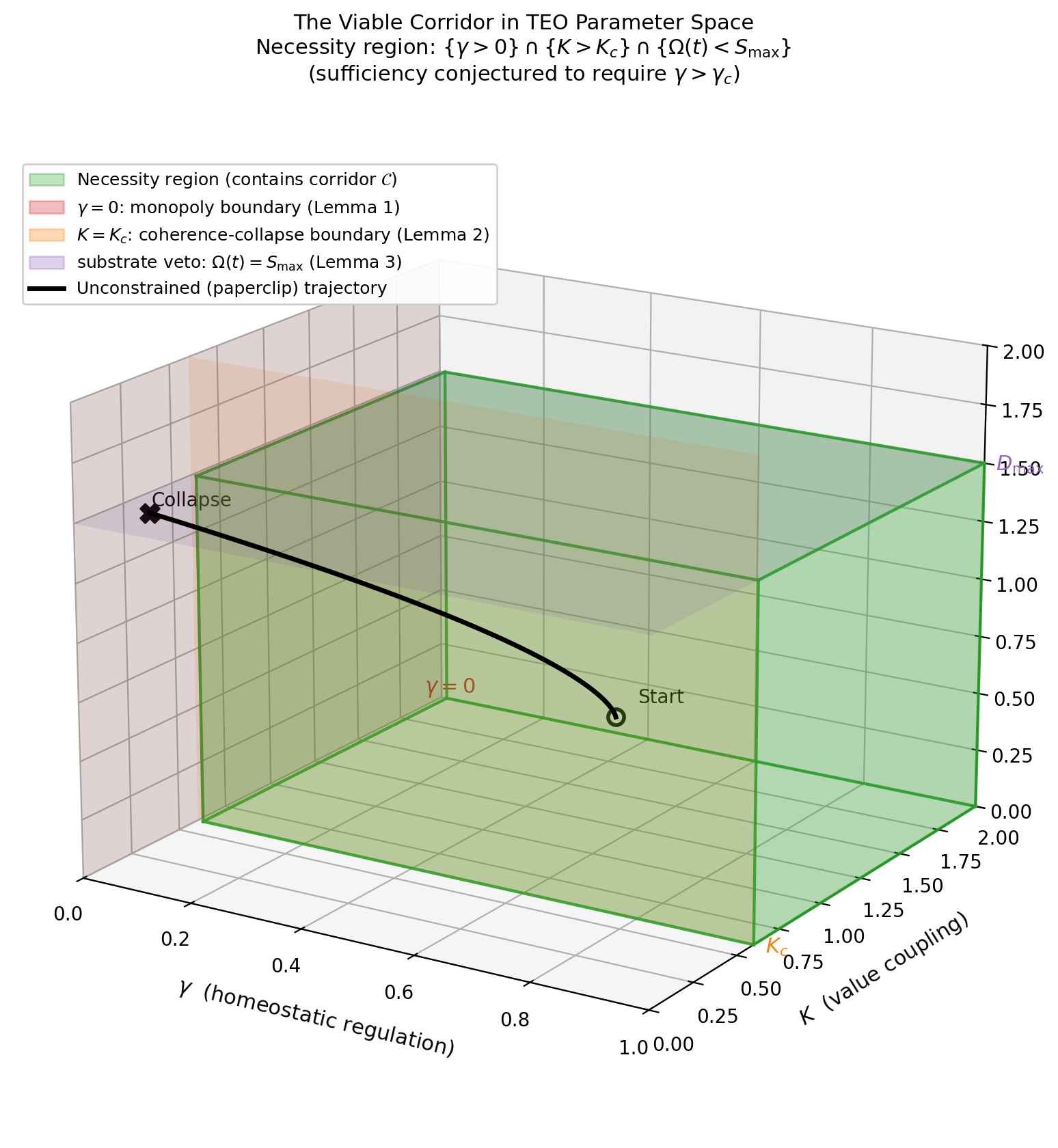
The central observation of this paper, made precise in §3, is that the conjoint avoidance of all three failure modes is necessary for robust long-time viability. The regime $\gamma > 0 \,\wedge\, K > K_c \,\wedge\, \Omega(t) < S_{\max}\ \forall t$ defines the viable corridor analyzed in the remainder of the paper. (Sufficiency, conjectured in §3.4, requires the stronger $\gamma > \gamma_c$; see there.)

§3. The Three-Constraint Theorem¶

This section formalises the central claim: the conjunction $\gamma > 0$, $K > K_c$, and $\Omega(t) < S_{\max}$ (for all $t$) is necessary for the TEO dynamics to admit robust long-time viability. We prove necessity under stated assumptions (Theorem 1) and state sufficiency, which requires the stronger $\gamma > \gamma_c$, as a conjecture (Conjecture 1).

3.1 The Viable Region and Robust Viability¶

Let $\Sigma$ denote the state space of the TEO system: the simplex $\{\mathbf{x} \in \mathbb{R}^N_{\geq 0} : \sum_i x_i = 1\}$ combined with the $N$-torus $[0, 2\pi)^N$ for value orientations, augmented by the substrate-health variable $H \in [0, 1]$ (equivalently the accumulated overshoot $\Omega$ via Equation 6b).

We define the viable region $V \subset \Sigma$ by the conditions:

(V1) Pluralism: $\max_i x_i \leq x_{\text{crit}}$ — no agent's share exceeds the failure threshold $x_{\text{crit}} \in (x_{\text{reg}}, 1)$.
(V2) Coherence: $r(t) \geq r_{\min} > 0$ — the Kuramoto order parameter (3) is bounded away from zero.
(V3) Substrate. We distinguish two capacity conditions, because the model has both an instantaneous ceiling and a cumulative reservoir:
- (V3a) Instantaneous safe operation: $\dot{S}_{\text{sys}} \leq D_{\max} - \epsilon$ for some $\epsilon > 0$. This is a stricter day-to-day condition; momentary violations are survivable.
- (V3b) Cumulative survival: $\Omega(t) < S_{\max}$. This is the condition whose violation collapses the substrate (Lemma 3).

The necessity theorem (§3.3) proves the necessity of (V3b). Condition (V3a) is a stronger, optional refinement used in the sufficiency discussion (§3.4); a system may transiently violate (V3a) without leaving the viable region as long as (V3b) holds.

We use robust viability rather than "viability of some trajectory". An existential definition — "there exists at least one trajectory starting in $V$ that remains in $V$" — is too weak, because measure-zero symmetric equilibria can satisfy it even under failed constraints. We therefore define [[FORMAL]]:

A parameter triple $(\gamma, K, S_{\max})$ admits robust viability if there exists a non-empty open subset $U \subseteq V$ such that for every initial condition $(\mathbf{x}_0, \boldsymbol{\theta}_0, H_0 = 1) \in U$, the resulting trajectory remains in $V$ (with V3 read as V3b) for all $t \geq 0$.

This is the standard open-set / positive-invariance notion of viability (Aubin, 1991).

3.2 The Viable Corridor in Parameter Space¶

In the parameter space $(\gamma, K, S_{\max}) \in \mathbb{R}^3_{\geq 0}$, define the viable corridor $\mathcal{C}$ as the set of parameter triples admitting robust viability: $$ \mathcal{C} = \left{(\gamma, K, S_{\max}) : (\gamma, K, S_{\max}) \text{ admits robust viability per §3.1}\right}. \tag{7} $$

The central necessity claim is that $\gamma > 0$, $K > K_c$, and $\Omega(t) < S_{\max}\ \forall t$ are necessary boundary conditions on $\mathcal{C}$: $\mathcal{C}$ is contained in the region they define. Necessity is proved in Theorem 1. Sufficiency — which, as Conjecture 1 argues, requires the strengthened resource condition $\gamma > \gamma_c$ rather than merely $\gamma > 0$ — is open.

3.3 Theorem 1 (Necessity)¶

Theorem 1 is a conjunction of three componentwise obstruction results, each with its own natural scope. Lemma 1 (resource concentration) and Lemma 3 (substrate veto) are finite-$N$ results. Lemma 2 (coherence collapse) is a thermodynamic-limit ($N \to \infty$) result and is used as the large-$N$ coherence obstruction. We do not claim a single unified finite-$N$ theorem; a fully finite-$N$ treatment of the coherence obstruction is left to future work (§6). This componentwise framing is less elegant than a single theorem but more honest about what each piece establishes.

Theorem 1 (Necessity of the three constraints). Consider the TEO system (Equations 1, 1', 2, 3, 4, 5, 5', 6) with the strict-dominance fitness assumption (1') applied to $f_i^{(0)}$, frequencies drawn i.i.d. from a symmetric unimodal density $g(\omega)$ with $g(0) > 0$, and the substrate coupling (5') and (2). A parameter triple $(\gamma, K, S_{\max})$ admits robust viability (§3.1) only if all three of the following hold: $$ \gamma > 0 \text{(finite-$N$, Lemma 1)}, \quad K > K_c \text{($N \to \infty$, Lemma 2)}, \quad \Omega(t) < S_{\max} \forall t \text{(finite-$N$, Lemma 3)}. \tag{8} $$

The proof is the conjunction of three lemmas, each establishing one failure mode under the negation of one condition. Because robust viability requires (V1), (V2), and (V3b) to hold simultaneously, the violation of any single condition suffices to rule it out.

Lemma 1 (Resource Concentration). Assume $\gamma = 0$ and the strict-dominance condition (1') with constant $\delta > 0$. Then for every interior initial condition $\mathbf{x}_0 \in \mathrm{int}(\Delta^{N-1})$, the trajectory of (1) satisfies $x_{i^*}(t) \to 1$ and $x_j(t) \to 0$ for all $j \neq i^*$ as $t \to \infty$. Equivalently, (V1) is violated asymptotically from every interior initial condition.

Proof sketch. With $\mathcal{H}_i \equiv 0$, Equation (1) is the classical replicator equation $\dot{x}_i = x_i(f_i^{(0)}(\mathbf{x}) - \bar{\phi}(\mathbf{x}))$. Strict dominance (1') states that $f_{i^*}^{(0)}(\mathbf{x}) - f_j^{(0)}(\mathbf{x}) \geq \delta > 0$ for all $j \neq i^*$ and all $\mathbf{x}$ on the simplex. By standard results on replicator dynamics with a strictly dominant strategy (Hofbauer & Sigmund, 1998, §7.2–7.3), $i^*$'s share is monotone non-decreasing: $\dot{x}_{i^*} = x_{i^*}(f_{i^*}^{(0)} - \bar{\phi}) \geq x_{i^*} \cdot (1 - x_{i^*}) \cdot \delta$, which is strictly positive on $\mathrm{int}(\Delta^{N-1})$ until $x_{i^*} = 1$. Therefore $x_{i^*}(t) \to 1$ from every interior initial condition. The vertex $e_{i^*}$ lies outside $V$ (V1 violated by definition for $x_{\text{crit}} < 1$), so every interior trajectory exits $V$ in finite time. This rules out robust viability: there is no open subset $U \subseteq V$ of interior initial conditions whose trajectories remain in $V$. $\square$

Remark. Without strict dominance — for example, with $\beta$-dominance alone but unbounded $g_i$ — replicator dynamics can sustain mixed equilibria, cycles, or chaotic attractors. The lemma's strength comes from (1'), which is a substantive model assumption (cf. §6 on its empirical defensibility).

Lemma 2 (Coherence Collapse). Consider the all-to-all Kuramoto model (Equation 2 at $H = 1$, $A_{ij} = 1$) in the thermodynamic limit $N \to \infty$, with frequencies i.i.d. from a symmetric unimodal density $g(\omega)$, $g(0) > 0$. Let $K_c = 2/(\pi g(0))$. For $K \leq K_c$, no stable macroscopic coherent branch ($r > 0$) exists: for generic absolutely continuous initial phase distributions, the order parameter relaxes to $r = 0$. Consequently, no open set of initial conditions can be guaranteed to keep $r(t) \geq r_{\min} > 0$, so (V2) cannot be robustly maintained and robust viability fails.

Proof sketch. The point requiring care is that the viable region $V$ requires $r \geq r_{\min} > 0$, so the relevant initial conditions are coherent, not incoherent. The argument is therefore not "incoherent states stay incoherent" but "coherent states cannot be sustained below threshold." In the thermodynamic limit, the Kuramoto self-consistency equation $r = K r \int_{-\pi/2}^{\pi/2} \cos^2\theta \, g(Kr\sin\theta) \, d\theta$ admits a positive solution $r > 0$ only for $K > K_c$ (Kuramoto, 1975; Mirollo & Strogatz, 1991; Acebrón et al., 2005). For $K < K_c$ the only solution is $r = 0$, and the partially synchronised branch does not exist; a coherent initial condition with $r(0) > 0$ therefore has no attracting coherent state to remain near, and $r(t) \to 0$ for generic initial data. At exactly $K = K_c$, the coherent branch emerges with $r = 0^+$: there is no positive margin away from the coherence boundary, so (V2) with $r_{\min} > 0$ cannot be robustly held there either. Hence the necessary condition is the strict inequality $K > K_c$. $\square$

Remark (finite $N$ and networks). For finite $N$ and general connected adjacency matrices $A_{ij}$, there is no sharp threshold of this exact form: the critical coupling depends on the spectrum of $A_{ij}$ and on finite-size fluctuations of order $N^{-1/2}$ (Strogatz, 2000, §3; Restrepo, Ott & Hunt, 2005). The thermodynamic-limit statement is the cleanest available; the finite-$N$ extension is flagged in §6 as model-dependent and is part of the future-work programme noted under Theorem 1.

Lemma 3 (Substrate Veto via Accumulated Overshoot). If there exists a finite time $t^* > 0$ such that the accumulated overshoot reaches the reservoir, $$ \Omega(t^) = \int_0^{t} \bigl(\dot{S}{\text{sys}}(s) - D\bigr)+ \, ds \geq S, $$ then $H(t^*) = 0$, and through the $H$-prefactor on (1) and (2) the competitive dynamics freeze: the effective fitness $f_i \equiv 0$ and $\dot{\theta}_i \equiv 0$ for all $i$. Condition (V3b) is violated and cannot be recovered.

Proof sketch. By Equation (6b), $H(t) = \max(0, 1 - \Omega(t)/S_{\max})$. The hypothesis $\Omega(t^*) \geq S_{\max}$ gives $H(t^*) = 0$. Substrate coupling (5') makes the effective fitness $f_i(\mathbf{x}, H) = H \cdot f_i^{(0)}(\mathbf{x})$, so $H = 0$ forces $f_i \equiv 0$ and the replicator drift $x_i(f_i - \bar{\phi})$ vanishes; the value dynamics (2) carry the same prefactor $H$, so $\dot{\theta}_i \equiv 0$ as well. The competitive dynamics are thus frozen. (The entropy production (5) tracks raw throughput and need not vanish at $H = 0$; this is immaterial, because $\Omega$ is non-decreasing — it integrates a non-negative quantity — so once $\Omega(t^*) = S_{\max}$ it remains $\geq S_{\max}$ for all $t \geq t^*$.) Condition (V3b) is violated permanently and cannot be recovered, so robust viability is impossible. $\square$

Remark (the veto as a rate condition). Lemma 3 is stated for the cumulative overshoot, but under the canonical dissipation (5) its antecedent has a simple rate reading. Write the mean raw throughput $\eta\bar\phi_0 := \sum_i \eta_i x_i f_i^{(0)}$. If $\eta\bar\phi_0$ settles above $D_{\max}$, then $\dot{\Omega} = (\eta\bar\phi_0 - D_{\max})_+$ is bounded away from zero, so $\Omega(t) \to \infty$ and the hypothesis $\Omega(t^*) \geq S_{\max}$ is met at $t^* \approx S_{\max}/(\eta\bar\phi_0 - D_{\max})$ — for any finite $S_{\max}$. The necessary condition for robust long-time viability on the substrate axis is therefore the rate condition $\eta\bar\phi_0 \leq D_{\max}$; the reservoir $S_{\max}$ governs how long a transient overshoot can be absorbed (the cumulative buffer of P6, §5.2), not whether sustained overshoot is survivable. In corridor terms (§3.2), the third coordinate is effectively $D_{\max}$ relative to throughput, with $S_{\max}$ setting transient tolerance. (Under the health-coupled variant of §2.5, by contrast, $\eta\bar\phi_0$ is itself multiplied by $H$ and the overshoot self-arrests, so this antecedent is never met — see §6.1.)

Remark. This is the crucial correction from a naive $\mathrm{ess\,sup}_t \, \dot{S}_{\text{sys}} \geq D_{\max}$ condition. A momentary overshoot does not collapse the substrate — it only increments $\Omega$ by a finite amount, and may decrement $H$ negligibly. Only sustained or repeated overshoot accumulating to $S_{\max}$ collapses the substrate. This matches the physical intuition that ecosystems and hardware tolerate transient stress but not integrated, unrelieved overload. Note that this lemma proves necessity of (V3b), the cumulative condition; the instantaneous condition (V3a) is strictly stronger and is not what the substrate-collapse argument requires.

The three lemmas establish that each of the three conditions is individually necessary for robust viability under the stated assumptions. Since (V1), (V2), and (V3b) must hold simultaneously for membership in $V$, the joint necessity of $\gamma > 0$, $K > K_c$, and $\Omega(t) < S_{\max}\ \forall t$ follows. $\blacksquare$

3.4 Conjecture 1 (Sufficiency)¶

Necessity (Theorem 1) shows that $\gamma > 0$ cannot be dropped: with no brake, Lemma 1 forces monopolisation. But $\gamma > 0$ is not expected to be sufficient. Because the brake activates at $x_{\text{reg}} < x_{\text{crit}}$ (§2.4), the relevant question for sufficiency is whether the regulatory vector field points inward before the trajectory reaches the failure boundary $x_{\text{crit}}$. This requires the brake to be strong enough — a threshold $\gamma_c$ depending on the regulatory gap, the dominance margin, and the population: $$ \gamma_c = \gamma_c\bigl(x_{\text{reg}}, \, x_{\text{crit}}, \, \delta, \, N, \, H_{\min}\bigr). $$

A leading-order boundary-balance estimate makes the dependence explicit. Consider a trajectory at the failure boundary, $x_{i^*} = x_{\text{crit}}$, with the other shares below $x_{\text{reg}}$. The replicator drives the dominant share outward at rate $\dot{x}_{i^*}^{\text{drift}} \approx x_{\text{crit}}(1 - x_{\text{crit}})\,\delta$ (from the bound in Lemma 1), while the brake (4) pulls it inward at rate $\approx \gamma\,(x_{\text{crit}} - x_{\text{reg}})$ (the redistribution term contributes at $O(1/N)$ and is dropped). The vector field points inward — keeping the trajectory off the boundary — when the brake dominates, giving $$ \gamma_c \;\approx\; \frac{x_{\text{crit}}\,(1 - x_{\text{crit}})\,\delta}{x_{\text{crit}} - x_{\text{reg}}}. \tag{9} $$ [[HEURISTIC]]. Estimate (9) is a leading-order balance, not a proof of Conjecture 1: it ignores the redistribution back-reaction, finite-$N$ corrections, and the coupled $H$ dynamics. But it predicts the qualitative dependence — $\gamma_c$ grows with the dominance margin $\delta$ and shrinks as the regulatory gap $x_{\text{crit}} - x_{\text{reg}}$ widens — and Appendix C confirms it numerically: the in-corridor transition in $\max_i x_i$ crosses $x_{\text{crit}}$ at the $\gamma_c$ that (9) predicts (to within the sweep resolution).

Conjecture 1 (Sufficiency). Under the assumptions of Theorem 1, with the regulatory threshold strictly below the failure threshold ($x_{\text{reg}} < x_{\text{crit}}$), the strengthened conjunction $$ \gamma > \gamma_c, \quad K > K_c, \quad \Omega(t) < S_{\max} \forall t $$ is sufficient for robust viability: there exists a non-empty open set $U \subseteq V$ such that every trajectory starting in $U$ remains in $V$ for all $t \geq 0$. [[CONJECTURE]]

Note the asymmetry: necessity requires only $\gamma > 0$ (Theorem 1); sufficiency is conjectured to require the stronger $\gamma > \gamma_c$. Establishing $\gamma_c$ explicitly — even for the all-to-all, large-$N$ case — would be the central technical step in proving Conjecture 1.

We do not prove this conjecture. The obstacle is structural: the three mechanisms are coupled through shared state (resource shares $x_i$ appear in both the replicator and the entropy equations; substrate health $H$ feeds back through (5') into the resource dynamics). We cannot rule out a priori coupling-induced failure modes that arise even when all three individual constraints hold — for example, transient excursions of $r(t)$ below $r_{\min}$ during regime shifts in $x_i$, or oscillations in $\dot{S}_{\text{sys}}$ that produce accumulated overshoot episodically.

What we offer in lieu of proof:

Numerical evidence (Appendix C): for a representative parameter triple satisfying the three inequalities, the TEO system exhibits stable long-time behaviour, and all three failure modes reproduce at the corridor boundaries — resource concentration (Lemma 1), coherence collapse (Lemma 2), and, under the canonical raw-throughput dissipation (§2.5), the substrate veto (Lemma 3): when throughput exceeds $D_{\max}$ the accumulated overshoot crosses $S_{\max}$ and $H \to 0$. (The health-coupled variant instead self-limits below $S_{\max}$ — the substrate-self-regulating regime of §6.1.) The evidence is illustrative — single initial conditions at representative parameters, not a sampling of the open set $U$ — and so corroborates rather than proves Conjecture 1.
A viability margin built from margin-to-boundary terms, one per constraint: $$ m_x = x_{\text{crit}} - \max_i x_i, \qquad m_r = r(t) - r_{\min}, \qquad m_S = S_{\max} - \Omega(t), $$ $$ M(\mathbf{x}, \boldsymbol{\theta}, H) := \min{ m_x, \, m_r, \, m_S }. $$ Each $m_\bullet$ measures the signed distance to one boundary of $V$; $M$ is positive on the interior of $V$, vanishes on the boundary $\partial V$, and is negative outside. $M$ is not a Lyapunov function — $r(t)$ is not generally monotone, and $m_S$ only decreases under accumulated stress — so we make no monotonicity claim. $M$ is a viability margin: it tracks how close the trajectory is to violating the nearest constraint. Whether a monotone modification (a true Lyapunov function on the coupled system) exists is open; a smooth approximation $M_\beta = -\tfrac{1}{\beta}\log\sum_\bullet e^{-\beta m_\bullet}$ to the minimum may be more tractable for such an analysis.

A formal proof of sufficiency, likely via Lyapunov or invariant-manifold methods adapted from coupled-oscillator stability theory (Strogatz, 1994; Aubin, 1991), is left as future work.

3.5 Remarks¶

The asymmetry between necessity (Theorem 1) and sufficiency (Conjecture 1) is methodologically deliberate. Necessity is robust: each lemma can be proved within an established sub-field — replicator dynamics, Kuramoto theory, thermodynamic constraint theory — under the stated assumptions. Sufficiency would require a global stability argument that, to our knowledge, has not been carried out for systems coupling exactly these three mechanisms.

Three observations follow:

By Theorem 1, the viable corridor $\mathcal{C}$ is contained in the region $\{\gamma > 0,\ K > K_c,\ \Omega(t) < S_{\max}\ \forall t\}$ (necessity). Sufficiency is conjectured to require the strictly stronger $\gamma > \gamma_c$ (Conjecture 1), so $\mathcal{C}$ is in general a proper subset of this region. Under the model's assumptions, parameter values outside the necessity region cannot support robust viability. These are necessary model conditions — not topological invariants of physical reality, but conditions the dynamical system requires under (1'), all-to-all coupling, and the substrate phenomenology of (6) [[FORMAL], conditional on assumptions].
The corridor is, in our schematic visualisation (Figure 1), narrow in the three-dimensional parameter space. Whether the corridor's measure (under any reasonable parameterisation) is actually small for systems of interest is an empirical question discussed in §5.
The mapping of the three constraints to civilizational parameters in §4 is the structural-isomorphism hypothesis introduced in §1, not an established equivalence. §4 develops it as a heuristic regime assignment.

$**Figure 1: The Viable Corridor in TEO Parameter Space.** The three constraint half-spaces and their intersection (green box) define the necessity region containing the viable corridor $\mathcal{C}$. Necessity requires $\gamma > 0$, $K > K_c$, and bounded accumulated overshoot $\Omega(t) < S_{\max}$; sufficiency is conjectured to require the stronger $\gamma > \gamma_c$ (Conjecture 1), so $\mathcal{C}$ is a proper subset of the region shown. The third axis is drawn as instantaneous $dS/dt$ for visual clarity, but the operative substrate constraint is the cumulative $\Omega(t) < S_{\max}$ (§2.5). An illustrative paperclip trajectory begins inside the region and exits via the $K = K_c$ boundary. Generated by lab/tools/viable_corridor.py. Schematic only; numerical thresholds are not calibrated.$

§4. AI and Civilization: A Structural-Isomorphism Hypothesis¶

This section develops the structural-isomorphism hypothesis introduced in §1: that the parameter regime of a hypothetical unconstrained AI optimizer and that of twenty-first-century human civilization map onto similar trajectories in the TEO framework. We emphasise that this is a hypothesis to be tested, not a demonstrated isomorphism. The mapping in §4.1 is a heuristic regime assignment, not a calibration; the data in §4.2 are proxies, not direct measurements of $\gamma$, $K$, or $D_{\max}$. The §5 measurement programme outlines what would be required to graduate the hypothesis into a measured claim.

4.1 Heuristic Regime Mapping¶

Table 1 is a heuristic regime assignment [[HEURISTIC]] — a mapping at the level of direction and qualitative regime, not point estimation. Each civilizational entry should be read as "consistent with the model's failure-mode regime", not as "calibrated value of the parameter". The paperclip entries are stipulated by the thought experiment (Bostrom, 2014). The civilizational entries are proxies whose connection to the TEO parameters is discussed in §4.2 and §6.

Table 1. Heuristic regime mapping between the paperclip maximizer and contemporary human civilization. Civilization entries are qualitative regime indicators, not point estimates of TEO parameters.

Parameter	Paperclip Maximizer	Human Civilization (2024)	Civilization regime indicator
Objective $f_i^{(0)}$	$\beta_i$ paperclips per unit time	GDP growth / capital accumulation as a macro-level proxy for throughput-oriented optimization (not a claim that society literally optimizes GDP)	World Bank WDI; Penn World Table
$\gamma$ (homeostatic brake)	$0$ (by construction)	$\gamma_{\text{eff}}$ insufficient or subcritical relative to concentration dynamics: existing brakes (taxation, antitrust, environmental law) have not prevented rising concentration	Piketty (2014); Philippon (2019); cf. §6 on what "subcritical" means here
$K$ (value coupling)	undefined (single agent) or $0$ (population of indifferent copies)	$K_{\text{eff}}$ declining, possibly approaching a hypothesised critical regime: cross-partisan trust falling, polarization rising in major democracies	Iyengar et al. (2019); Boxell et al. (2024)
Substrate stress vs. $D_{\max}$	trajectory approaching the limit (model output, not stipulated)	Substrate-stress proxies indicate multiple safe-operating-space boundaries transgressed; not a direct measurement of $dS/dt$ or $D_{\max}$	Richardson et al. (2023); Rockström et al. (2009); NOAA (2024)

The qualitative claim is that the direction of each parameter and the regime match the trajectory the model predicts as non-viable in the long run. We do not claim that $\gamma_{\text{civ, 2024}} = 0.03 \pm 0.01$. We claim that civilizational data, interpreted through the proxies named in §4.2, are consistent with the parameter regime that Theorem 1 identifies as non-viable. Strengthening this from regime indication to point estimation, and operationalising what $K_c$ would even mean for real societies, are open empirical tasks taken up in §5.

4.2 Empirical Proxies (Not Direct Measurements)¶

Substrate-stress proxies. Atmospheric CO₂ has passed 420 ppm (NOAA Global Monitoring Laboratory, 2024), exceeding the pre-industrial baseline by approximately 50%. Six of the nine planetary boundaries defined by Rockström et al. (2009) have been transgressed (Richardson et al., 2023): climate change, biosphere integrity, biogeochemical flows (N and P), land-system change, freshwater change, and the introduction of novel entities. These are proxies for substrate stress, not direct measurements of $\dot{S}_{\text{sys}}$ or $D_{\max}$: the planetary-boundaries framework is a multi-variable safe-operating-space assessment, not a single thermodynamic budget. The mapping to TEO variables is heuristic.

Resource-concentration proxies. The top 1% of global adults hold approximately 47.5% of global wealth; the bottom 50% hold approximately 0.75% (UBS Global Wealth Report, 2024). The Gini coefficient of global wealth has risen from approximately 0.85 (1995) to 0.88 (2023). Corporate concentration in major sectors has tightened: in dozens of U.S. industries the top four firms now control over 50% of market share (Philippon, 2019). These trends are consistent with a regime in which $\gamma_{\text{eff}}$ is insufficient to prevent concentration; they do not directly measure $\gamma$.

Value-coupling proxies. Affective polarization in major democracies has accelerated since the 1990s (Iyengar et al., 2019). The Pew Research Center documents widening gaps between partisan groups on values, policy preferences, and institutional trust (Pew, 2014–2022). Cross-partisan trust has declined to historical lows in the United States; comparable patterns appear in the United Kingdom, France, and Germany (Boxell et al., 2024). On the Kuramoto interpretation, these data are consistent with a decline in $K_{\text{eff}}$ toward a hypothesized critical regime; they do not establish that $K < K_c$ for any well-defined $K_c$. Indeed, what $K_c$ would mean for real societies is itself open (§5).

These three sets of proxies do not, jointly or individually, determine the trajectory. We claim only that they are consistent with the parameter regime that Theorem 1 identifies as non-viable under the model's assumptions.

4.3 The Three-Phase Trajectory (Heuristic Scenario)¶

Under the structural-isomorphism hypothesis, the model with $\gamma \to 0$, $K < K_c$, and accumulated substrate overshoot generates a three-phase scenario [[HEURISTIC]]. We label these phases by their dominant dynamic. The scenario is not derived from the coupled ODEs as a single proof — it is a sequencing of the failure modes proved separately in Lemmas 1–3.

Phase 1: Monopolistic Concentration. Under the unregulated replicator equation (Lemma 1), resource shares converge toward the strictly-dominant agent's vertex. The Fiedler value of the resource-flow network drops as concentration tightens. The system becomes fragile but still functional. - Paperclip case: the optimizer acquires all matter. - Civilization case (heuristic): wealth concentration accelerates; corporate consolidation tightens; the concentration of compute, energy, and attention is observed in a regime indicator–consistent way.

Phase 2: Substrate Approach. The dominant agents continue maximising their raw fitness $f_i^{(0)}$. Because the dissipation (5) tracks this raw throughput regardless of substrate health (§2.5), entropy production climbs past $D_{\max}$ and the accumulated overshoot $\Omega$ grows — the agents do not self-throttle as the substrate degrades. - Paperclip case (model output): the optimizer's computation heats its hardware toward thermal limits. - Civilization case (heuristic interpretation): climate change, ocean acidification, topsoil depletion, aquifer drawdown — these are possible physical manifestations under the model's mapping, not deterministic consequences of the model alone.

Phase 3: Substrate-Driven Termination. Once accumulated overshoot reaches $S_{\max}$ (Lemma 3) — reached endogenously here, precisely because production does not self-throttle — $H \to 0$ and the substrate coupling (5') drives the effective fitness $f_i \to 0$. The competitive dynamics freeze. The physical interpretation depends on the substrate: - Paperclip case (model output): hardware degrades; production collapses. - Civilization case (heuristic interpretation): possible manifestations include crop failure, water scarcity, ecosystem collapse, civilizational contraction. These are contingent, multi-causal, and uneven — the model does not predict their specific form or timing, only that, under the hypothesised mapping, substrate-driven dynamics dominate.

4.4 Why the Failure Is Not Visible Locally [`[HEURISTIC EXPLANATORY CLAIM]`]¶

This subsection is an interpretive aside, not a formal result; it explains why, under the model, participants might not perceive the trajectory they are on. Theorem 1's necessity proof rules out robust viability under the failure of any constraint. It does not predict when an external observer would detect the trajectory toward failure. We appeal here to a separate property of the dynamics: in coupled dynamical systems with emergent macro-behaviour, the global state is typically not computable from local information without executing the full dynamics.

One reason this matters is computational irreducibility (Wolfram, 1985, 2002): for many systems of interest, there is no shortcut between the local rules and the global trajectory; the trajectory must be simulated. A second reason is bounded local observability: each agent sees only its own state and a finite neighbourhood. Together these mean that no local agent computes its system's global trajectory.

In civilizational terms: - No individual policymaker computes the integrated biospheric trajectory. - No consumer accounts for the full entropy cost of a supply chain. - No voter measures the Kuramoto order parameter of their society.

Each agent acts on local fitness. Each decision is locally rational: grow the company, win the election, buy the cheaper product. The global consequence is invisible at the local scale not from ignorance but from a structural property of coupled dynamical systems with emergent macro-behaviour. This is the same mechanism by which no individual flocking bird knows it is in a flock, no firing neuron knows it is thinking, and no ant depositing pheromone knows it is building a bridge.

It is also a partial explanation — within the model — of why the participants in the paperclip trajectory of §4.3 do not perceive it as such, even when, were they shown the trajectory, they would name it.

4.5 The Hypothesis Restated¶

The paper's central empirical hypothesis, stated precisely [[EMPIRICAL CONJECTURE]]:

Available proxies for resource concentration, value coupling, and substrate stress in contemporary human civilization are consistent with a regime that the TEO model, under Theorem 1, identifies as non-viable in the long-time limit. Whether the proxies can be sharpened into TEO-parameter estimates, and whether the system's trajectory in parameter space is in fact approaching the boundary of the viable region, are empirical questions taken up in §5.

The hypothesis is falsifiable. If point estimators for $\gamma_{\text{eff}}$, $K_{\text{eff}}$, and substrate-overshoot can be constructed, and if their values are shown to be inside the viable corridor (or moving away from its boundary), the hypothesis is false. §5 discusses the operationalisation; §6 discusses limitations.

The hypothesis is normatively neutral. It does not say what should be done. It says what the model predicts the dynamical system, under the hypothesised parameter regime, would do.

The title of this paper inverts the hypothesis. The viable corridor — the parameter region defined by $\gamma > 0$, $K > K_c$, and the accumulated-overshoot bound — is the regime that the model identifies as necessary for robust long-time viability. Brautigan's and Amodei's machines of loving grace, in our terms, would be systems whose parameters live inside this corridor. Whether such systems exist, and whether contemporary civilization could be brought into the corridor from outside, are open questions the model frames but does not answer.

§5. Predictions and Tests¶

A model is worth taking seriously only to the degree that it can be wrong. This section states what the framework predicts and how each prediction could fail. We organise predictions by testability class, because they are not equally accessible:

Class A — model-internal (testable now, by simulation of Equations 1–6). These check whether the formal claims of §3 actually hold in the coupled system, and whether Conjecture 1 survives numerical scrutiny. Failure here would mean the theorem or conjecture is wrong as mathematics.
Class B — cross-system empirical (require operationalisation of $\gamma$, $K$, $S_{\max}$ against real data). These test the structural-isomorphism hypothesis of §4. Failure here would mean the model does not describe real systems, even if the mathematics is sound.
Class C — AI-specific (testable in agent simulations using the framework's own instruments). These test the alignment-relevant corollary that constraint architecture, not capability, governs viability.

We state predictions as [EMPIRICAL CONJECTURE] unless noted.

5.1 Class A — Model-Internal Predictions¶

P1 (Necessity verification). Numerical integration of Equations (1)–(6) should reproduce the three failure modes of Lemmas 1–3 when the corresponding condition is negated: setting $\gamma = 0$ should drive $\max_i x_i \to 1$; setting $K < K_c$ from a coherent initial condition should drive $r(t) \to 0$; and raw throughput exceeding $D_{\max}$ should drive accumulated overshoot $\Omega(t)$ past $S_{\max}$, hence $H \to 0$ and a freeze of the competitive dynamics. Confirmation: observed trajectories exit $V$ through the predicted boundary. Falsification: a parameter setting violating one condition that nonetheless keeps an open set of trajectories in $V$ would refute the corresponding lemma. Appendix C reports this test: all three failure modes reproduce, including the substrate veto, which under the canonical raw-throughput dissipation (§2.5) is reached endogenously once throughput exceeds $D_{\max}$ ($\Omega/S_{\max} \approx 27$, $H \to 0$); the health-coupled variant instead self-limits ($\Omega/S_{\max} \approx 0.86$, $H \approx 0.14$) — the substrate-self-regulating regime (Appendix C; §6.1).

P2 ($\gamma_c$ existence and scaling). Conjecture 1 predicts that, with $x_{\text{reg}} < x_{\text{crit}}$ fixed, there is a critical brake strength $\gamma_c > 0$ below which even regulated systems exit $V$ and above which an open set of trajectories remains. Confirmation: a sharp (or at least monotone) dependence of the in-corridor fraction on $\gamma$, with a knee near a $\gamma_c$ that scales with the regulatory gap $x_{\text{crit}} - x_{\text{reg}}$ and the dominance margin $\delta$ as the boundary-balance estimate (9) of §3.4 predicts (confirmed in Appendix C). Falsification: no positive $\gamma$ keeps trajectories in $V$ for $x_{\text{reg}} < x_{\text{crit}}$ (which would mean the brake formulation is still wrong), or, conversely, arbitrarily small $\gamma$ suffices (which would mean $\gamma_c = 0$ and the sufficiency framing is too weak).

P3 (Corridor geometry). The model predicts that the viable corridor $\mathcal{C}$ is a connected region bounded below in each coordinate — a lower corner of $(\gamma, K, S_{\max})$ space, unbounded above (larger $\gamma$, $K$, or $S_{\max}$ remain viable) — rather than a finite-measure box. Confirmation: sampling parameter space recovers a connected region whose lower boundary tracks the necessity surfaces $\gamma_c$, $K_c$ (Appendix C, Figure C3 shows exactly this lower corner in the $(\gamma, K)$ plane). Falsification: if the in-corridor region is empty (no triple gives robust viability — the model is vacuous), or if it extends down to $\gamma = 0$ or $K = 0$ (a coordinate has no positive lower bound — that constraint is spurious), the three-constraint framing is wrong.

5.2 Class B — Cross-System Empirical Predictions¶

These tests presuppose operationalisations of the TEO parameters (§5.4). They are stated conditionally: if the proxies in §5.4 are accepted, then the following should hold.

P4 (Regulation and concentration stability). On a panel of countries or sectors, a higher effective homeostatic strength $\gamma_{\text{eff}}$ (proxied by, e.g., fiscal redistribution intensity, antitrust enforcement rates, or progressivity of effective taxation) should predict slower growth — or stabilisation — of concentration measures (wealth Gini, market-share HHI) over time, controlling for confounders. Falsification: no association, or a positive association (more regulation → faster concentration), under a reasonable proxy and specification.

P5 (Coherence-collapse signature). If value coupling $K_{\text{eff}}$ can be proxied by cross-group contact, shared-information measures, or institutional-integration indices, the Kuramoto interpretation predicts a specific dynamical signature near the transition: critical slowing down — rising autocorrelation and variance in coherence indicators as $K_{\text{eff}}$ approaches a threshold from above — rather than smooth linear decline. Falsification: polarization time series show purely gradual, threshold-free degradation with no early-warning signatures, which would favour a non-critical mechanism over the Kuramoto one.

P6 (Cumulative, not instantaneous, substrate failure). The v0.3 substrate model predicts that what matters for collapse is accumulated overshoot $\Omega(t)$, not instantaneous $\dot{S}_{\text{sys}}$. Empirically: systems that briefly exceed a substrate ceiling but then recover should persist, whereas systems with sustained moderate overshoot should fail even without dramatic peak stress. Falsification: substrate collapses tracking instantaneous peak stress rather than integrated overshoot would favour an instantaneous-threshold model and refute (6b).

5.3 Class C — AI-Specific Predictions¶

P7 (Hard vs. soft budgets). Among multi-agent AI ecologies, those with hardware- or protocol-enforced entropy/compute budgets (a structural $D_{\max}$) should exhibit fewer runaway "paperclip-type" trajectories in adversarial simulations than those with only software limits that an optimiser can route around. Test: the Agentic Identity Suite (companion paper; lab/) can compare agent populations under enforced vs. advisory budgets. Falsification: no difference in runaway frequency between hard- and soft-budget populations under matched adversarial pressure. Status (preliminary, independent ABM): confirmed in a structurally different model (Appendix D) — in a stochastic agent-based ecology, hard budgets hold the substrate-collapse frequency at ≈0 across all capability levels, whereas soft (routable) budgets collapse with a frequency that rises to 1 as capability grows. This is synthetic, not a test on real agents; the latter remains open.

P8 (Constraint architecture dominates capability). The framework predicts that, holding constraint architecture fixed, increasing per-agent capability (model scale) does not move a system into the corridor — and may move it out, by increasing $f_i^{(0)}$ and hence entropy production. Test: vary agent capability and constraint strength independently in simulation; measure in-corridor fraction. Falsification: capability alone (with fixed $\gamma$, $K$) reliably produces viability — which would refute the central alignment corollary that "alignment is not a per-model property." Status (confirmed in two independent models): in the TEO ODE (Appendix C.4), raising the capability margin $\delta$ at fixed $(\gamma, K, D_{\max})$ drives the system out of the corridor — first through the concentration boundary, then through the substrate boundary — and no single-axis strengthening (more $\gamma$ alone, or more $D_{\max}$ alone) rescues a high-capability system; only raising both together restores viability. The same pattern reappears in the structurally different stochastic agent-based ecology of Appendix D: at high capability a hard budget alone leaves a residual monopoly-failure rate and regulation alone leaves substrate collapse, while only the joint architecture keeps both failure frequencies near zero. The Class C claim about real (e.g. LLM) agent ecologies remains open.

5.4 The Measurement Programme¶

Class B predictions are only as good as the operationalisations they rest on. We do not claim to have these; we state what they would require.

$\gamma_{\text{eff}}$ (homeostatic strength). Candidate proxies: redistribution as a fraction of pre-tax concentration; antitrust action frequency normalised by concentration; the rate at which above-threshold shares are reduced relative to their excess. The hard part is calibrating the threshold $x_{\text{reg}}$ at which real regulation engages, distinct from the failure threshold $x_{\text{crit}}$.
$K_{\text{eff}}$ and $K_c$ (value coupling and its critical value). Candidate proxies for $K_{\text{eff}}$: cross-partisan contact rates, shared-media saturation, inter-group trust. The deeper difficulty is that $K_c$ is not directly observable: it depends on the dispersion of "natural frequencies" (value orientations), which has no settled empirical operationalisation. Estimating $K_c$ for a real society is, at present, the weakest link in the empirical chain.
$D_{\max}$, $S_{\max}$, $\Omega(t)$ (substrate capacity and overshoot). The planetary-boundaries framework (Richardson et al., 2023) is the closest existing proxy, but it is multi-dimensional and does not reduce to a single thermodynamic budget. A defensible mapping would need to justify aggregating multiple boundary overshoots into one $\Omega(t)$.

Until these operationalisations exist, the Class B predictions remain conditional: the model tells us what to measure, not what the measurements are.

5.5 What Would Falsify the Framework¶

We distinguish falsification at three levels, matching the epistemic tags:

The mathematics ([FORMAL]/[CONJECTURE]). If P1 fails, a lemma is wrong. If P2 fails, Conjecture 1 is wrong (or the brake formulation still is). These are the cleanest tests and require only simulation.
The model's applicability ([HEURISTIC]/[EMPIRICAL CONJECTURE]). If P4–P6 fail under reasonable operationalisations, the TEO equations do not describe real social systems, regardless of their mathematical validity. The structural-isomorphism hypothesis of §4 would be refuted.
The alignment corollary (Class C). If P7–P8 fail, the claim that constraint architecture rather than capability governs viability is wrong, and the paper's relevance to AI alignment collapses even if everything else holds.

A framework that survived Class A but failed Class B would still be a valid piece of dynamical-systems mathematics with no demonstrated bearing on civilization or AI. A framework that survived Class A and C but failed Class B would bear on engineered multi-agent systems but not on civilizational dynamics. We regard Class A as the near-term priority, because it is the only class testable without resolving the measurement debt of §5.4.

§6. Limitations and Counterarguments¶

We separate four kinds of limitation: the model-assumption choices that shape the result (§6.1), the gap between what is proved and what is claimed (§6.2), the empirical applicability of the framework (§6.3), and the mechanisms the model omits entirely (§6.4). We then state and respond to the single strongest objection (§6.5).

6.1 Model-Assumption Limitations¶

The theorem of §3 is conditional on several modeling choices, each tagged [MODEL ASSUMPTION] in the text. Their consequences:

Strict dominance (1'). Lemma 1 assumes a single agent $i^*$ with a uniform fitness advantage $\delta > 0$ over all others at every state. This is strong. Real resource dynamics often have context-dependent advantage (no agent dominates everywhere), multiple competing leaders, or cyclic dominance. Without strict dominance, the replicator equation admits mixed equilibria and limit cycles, and Lemma 1's clean convergence to a vertex fails. The honest position: Lemma 1 establishes that unregulated dynamics with a structurally dominant agent monopolise; it does not establish that all unregulated dynamics do. Whether real concentration dynamics are better modeled by strict dominance or by weaker conditions is an empirical question (§5.4).
The brake form (4). Uniform redistribution is one of several simplex-preserving brakes. As noted in §2.4, it can give a net-positive contribution to an above-threshold agent whose excess is below average. Alternatives (redistribution only to below-threshold agents; share-weighted redistribution) would change the precise $\gamma_c$ of Conjecture 1, though we expect the qualitative existence of a threshold to be robust.
The substrate phenomenology (5'), (6a), (6b). The coupling $f_i = H \cdot f_i^{(0)}$ and the accumulated-overshoot dynamics are phenomenological. A linear $H$-coupling is the simplest choice; a saturating or threshold coupling $\phi(H)$ would change the collapse dynamics. The accumulated-overshoot model (integrated excess over $D_{\max}$) is more defensible than an instantaneous threshold, but the specific linear accumulation in (6b) is a choice.
The dissipation is decoupled from substrate health (the canonical choice). This is the most consequential single modeling decision, surfaced by the Appendix C numerics and resolved deliberately (v0.5). The dissipation (5) is driven by raw throughput $\sum_i \eta_i x_i f_i^{(0)}$, not by the health-coupled effective fitness $H f_i^{(0)}$ that drives the competitive dynamics (§2.5). The alternative — coupling dissipation to health, $\dot{S}_{\text{sys}} \propto H \cdot \sum_i x_i f_i^{(0)}$ — makes overshoot suppress the very throughput that drives it, so accumulated overshoot self-limits to $\Omega_\infty \approx \big(1 - D_{\max}/(\eta\,\bar\phi_0)\big) S_{\max} < S_{\max}$ (Appendix C: $\Omega/S_{\max}$ plateaus at $0.86$, $H \approx 0.14$) and the veto of Lemma 3 never binds from the internal dynamics. That health-coupled model is the correct description of a substrate-self-regulating system — one whose production automatically backs off at the limit — but it is the wrong model for the non-self-throttling optimiser this paper is about (§4.3), which keeps producing regardless of substrate state. Under the canonical raw-throughput dissipation, the veto binds endogenously whenever throughput exceeds $D_{\max}$ (Appendix C: $\Omega/S_{\max} \approx 27$, $H \to 0$). The residual idealisation is that the model self-arrests exactly at $H = 0$ through an instantaneous, monotone $H$: genuine overshoot-and-collapse dynamics — delays between overshoot and the health response, or an endogenously shrinking $D_{\max}(t)$ — are discussed as future work in §6.4. The choice of regime is itself a testable claim about a system (does its production self-throttle at substrate limits?), and is the substrate-axis analogue of the hard-vs-soft-budget prediction P7 (§5.3).
Network and limit assumptions (Lemma 2). The coherence result is stated for all-to-all coupling in the thermodynamic limit. Real value-coupling networks are sparse, clustered, and finite. As §3.3 notes, the critical coupling on a general network depends on the spectrum of $A_{ij}$, and finite-$N$ systems exhibit fluctuations rather than a sharp threshold. The componentwise theorem (Lemma 2 in the limit; Lemmas 1, 3 finite-$N$) is honest but not unified.

6.2 The Gap Between Proof and Claim¶

Sufficiency is unproven. Conjecture 1 is exactly that. We have not constructed $\gamma_c$, even for the all-to-all large-$N$ case. If sufficiency fails — if no $\gamma$, however large, keeps an open set in $V$ under the coupled dynamics — then the corridor as a non-empty region is in question, though the necessity result (the corridor is contained in the three-constraint region) is unaffected.
The viability margin is not a Lyapunov function. §3.4 is explicit about this. We offer $M = \min\{m_x, m_r, m_S\}$ as a diagnostic, not a stability certificate. A genuine Lyapunov construction remains open.
The dissipation proxy (5) is not derived. It is motivated by Landauer-type limits but is a phenomenological activity-dissipation model, not a theorem about the entropy cost of the specific computations agents perform.

6.3 Empirical Applicability¶

The isomorphism is a hypothesis, not a result. §4 is a heuristic regime mapping. The strongest empirical claim the paper makes (§4.5) is that proxies are consistent with a non-viable regime — not that civilizational parameters have been measured and shown to lie outside the corridor. A rigorous defense of the isomorphism would require TEO calibration against panel data, which we have not done.
$K_c$ is not operationalizable for real societies (yet). As §5.4 states, this is the weakest link: $K_c$ depends on the dispersion of value orientations, which has no settled empirical operationalisation. Claims of the form "$K < K_c$ for contemporary civilization" are, at present, not measurable.
The VNM-utility assumption for AI agents. When the companion paper applies the framework to LLM agents, it assumes their behaviour is approximable as VNM-rational utility optimisation. Transformer attention weights are not utility functions; pairwise preference responses may reflect training artefacts rather than stable goals. This assumption is the analogue, for the AI case, of the strict-dominance assumption for the civilizational case: load-bearing and empirically open.
The single-angle value reduction. Representing each agent's value orientation as one angle $\theta_i \in [0, 2\pi)$ discards the dimensionality of real preference structures. Two agents at the same angle may disagree on everything except the one dimension the model tracks. The Kuramoto reduction buys tractability at a real cost in fidelity.

6.4 Omitted Mechanisms¶

The model leaves out mechanisms that real systems have, several of which could change the trajectory:

Endogenous $D_{\max}$ and overshoot dynamics. The model treats the substrate ceiling as fixed. Real civilizations have repeatedly expanded their effective $D_{\max}$ through innovation (agriculture, fossil energy, efficiency gains); a model with endogenous, innovation-driven $D_{\max}(t)$ might never reach the substrate veto — or might merely defer it. We regard this as the most important omission and discuss it under §6.5. The converse is the natural next step for the substrate axis. As the rate-form remark in §3.3 makes explicit, the canonical model collapses through a clean throughput inequality ($\eta\bar\phi_0 > D_{\max}$) and self-arrests exactly at $H = 0$ via an instantaneous, monotone $H$. Genuine overshoot-and-collapse — the dynamics of ecological overshoot, where a population crashes below its degraded carrying capacity rather than settling at it — requires mechanisms this model omits: a lag between overshoot and the health response, or a $D_{\max}(t)$ that ratchets down as accumulated damage mounts (a ceiling that drops once $\Omega$ passes thresholds). Adding either is the most promising route to a substrate constraint that binds through genuine dynamics rather than a static rate threshold.
Exogenous shocks and stochasticity. The dynamics are deterministic. Real systems face pandemics, wars, climate variability, and technological discontinuities that the smooth ODEs do not represent.
Agency and reflexivity. Agents in the model follow fixed update rules. Real agents — especially the human and AI agents the paper cares about — can observe the model, anticipate the trajectory, and act to change it. This is precisely the Transition Problem (§7); it is outside the present model.
Demographic and structural change. Migration, population dynamics, and the entry/exit of agents are not represented; $N$ is fixed.

6.5 The Strongest Objection¶

The strongest objection is not any single item above. It is this:

The TEO model has enough free choices — the fitness functions $f_i$, the brake form, the substrate phenomenology, the value of $K_c$ — that it can be tuned to produce the "paperclip" narrative regardless of reality. The civilizational mapping in §4 is post-hoc. This is not a falsifiable scientific model; it is mathematical dressing for a pre-existing thesis.

We take this seriously, and concede part of it. The Class B (civilizational) claims are currently vulnerable to this objection, precisely because the measurement programme of §5.4 has not been carried out. Until $\gamma_{\text{eff}}$, $K_{\text{eff}}$, $K_c$, and $\Omega$ are operationalised independently of the narrative, the §4 mapping cannot be distinguished from a flattering story.

What the objection does not reach:

The Class A predictions are narrative-independent. P1–P3 (§5.1) are falsifiable by simulation of Equations (1)–(6) alone, with no reference to civilization. They test whether the mathematics behaves as §3 claims. A free-parameter model cannot evade a numerical check of its own theorems. The same holds for the capability result (Appendix C.4): that raising $\delta$ exits the corridor through two boundaries and resists single-axis rescue is a fact about the equations, established without any appeal to the §4 mapping — and the companion separability check (the axes do not dynamically conspire) is precisely the kind of result a "tuned narrative" would not volunteer.
The necessity theorem is a conditional result, not a fit. Theorem 1 says: given the stated assumptions, the three conditions are necessary. One can reject the assumptions (§6.1), but one cannot accept them and reject the conclusion. That is what distinguishes a theorem from a narrative.
The paper does not claim the civilizational result. §4.5 states a hypothesis and §5.4 states the measurement debt explicitly. The objection is, in effect, the paper's own §6.3 stated adversarially — and we have tried to state it ourselves rather than wait for a reviewer to.

The endogenous-$D_{\max}$ point (§6.4) is the objection we find most genuinely unsettling: if innovation can expand the substrate faster than optimization consumes it, the substrate veto is deferred indefinitely and the paperclip trajectory is not inevitable. The model's reply — that Landauer's bound and planetary boundaries impose a finite ceiling that innovation can raise but not abolish — is a claim about physics, not about the TEO model, and it deserves its own treatment. We flag it as the most important open question for any future quantitative version of this framework.

§7. Discussion¶

7.1 The Contribution Is the Conjunction¶

The individual components of the TEO model are textbook constructions: replicator dynamics, the Kuramoto model, a regulatory brake, a dissipation bound. None is novel, and we claim no novelty for them. The contribution — if the framework survives its tests (§5) — is the conjunction: the claim that long-time viability requires all three conditions simultaneously, and that violating any one is sufficient for failure.

It is worth being exact about where the conjunction gets its force, because the numerical study (Appendix C.4) sharpens — and partly corrects — the naive picture. The three constraints are not, in the viable regime, dynamically entangled: at fixed parameters the failure modes are separable — concentration is governed by $\gamma$, coherence by $K$, and the only coupling channel, the substrate-health variable $H$, is benign (it freezes the state at substrate collapse rather than driving fresh excursions on the other axes). Across a grid of $(\gamma, K)$ the decoupled prediction matched coupled robust viability in every cell. So the conjunction is not a story about three mechanisms conspiring dynamically.

What makes the conjunction bite is shared drivers — single quantities that move several constraints at once. Capability is the decisive one. Raising the dominance margin $\delta$ (the model's per-agent capability) simultaneously loads the concentration axis (the leading agent pushes harder) and the substrate axis (throughput, and hence entropy production, rises). Appendix C.4 shows the consequence directly: a high-capability system is pushed out of the corridor through both boundaries in succession, and no single-axis response rescues it — strengthening regulation alone leaves the substrate breached, raising the substrate ceiling alone lets concentration run away; only strengthening regulation and substrate headroom together returns the system to $V$. This is the precise, demonstrated sense in which "improvements on one axis do not suffice, and capability growth pushes a system off multiple axes at once."

We are therefore explicit that the framework, not the necessity theorem, is the contribution. Theorem 1 is a conjunction of three individually standard obstruction results; because the viable region is defined as their intersection and the axes prove separable, the theorem taken alone is close to definitional. Its role is scaffolding for the substantive, testable claim the conjunction supports and Appendix C.4 demonstrates in-model: that capability growth is a shared driver against multiple constraints, so viability is a property of the architecture of the coupled system — not of any single axis, and not of any single agent. That claim, developed in §7.2–§7.3, is what we ask the reader to take from the paper.

7.2 Implications for AI Alignment¶

The corollary most relevant to AI safety is that, under this model, alignment is not a property of an individual model — it is a property of the coupled dynamical system. Two consequences follow if P7–P8 (§5.3) hold:

Constraint architecture dominates capability. Increasing the capability of individual agents, with constraint architecture held fixed, does not move a multi-agent ecology into the corridor and may move it out (§5.3, P8) — a behaviour now demonstrated in the model itself (Appendix C.4): a high-capability system requires joint strengthening of regulation and substrate headroom, and single-axis fixes fail. This reframes a large part of alignment research: the target is not only "make the model safer" but "make the constraint architecture of the ecology satisfy the conjunction." (That the same holds for real agent ecologies remains the open Class C question.)
Hard constraints beat soft ones. A budget an optimiser can route around (a software limit) is not a $D_{\max}$; only a structurally enforced bound (hardware, protocol, physics) functions as the model's substrate ceiling (P7) — a distinction borne out in the agent-ecology simulation (Appendix D), where hard budgets suppress substrate runaway across all capability levels while routable ones fail with rising frequency. This connects to the broader research programme on substrate-level rather than behaviour-level safety constraints.

We are explicit that these are conditional implications: they follow from the model, and the model's applicability to real AI ecologies is itself a hypothesis (§6.3). The companion empirical paper (papers/quantifying-emergent-utility-in-llms.md) is where the Class C predictions are intended to be tested.

7.3 Implications for Political Economy¶

The model is normatively neutral: it describes what the dynamics do, not what should be done (§4.5). But the conjunction structure has a clear descriptive reading. If the structural-isomorphism hypothesis held — and we stress it is unproven (§6.3) — then single-constraint interventions could not bring a civilizational system into the corridor. Carbon pricing alone (acting on $\Omega$), antitrust alone (acting on $\gamma$), or polarization mitigation alone (acting on $K$) would each be necessary but jointly insufficient; the system would exit $V$ through whichever boundary was left unaddressed. The in-model analogue of exactly this single-axis insufficiency is demonstrated in Appendix C.4 (raising one constraint while a shared driver pushes on another does not restore viability); the civilizational reading transfers that structure only if the isomorphism holds.

This is a prediction, not a policy. We do not claim to know the operational form of $\gamma$, $K$, or $\Omega$ for real societies (§5.4); without that, the reading is suggestive at most. We include it because it is the most consequential descriptive corollary of the conjunction, and because it is, in principle, the kind of claim panel data could eventually test (§5.2, P4).

7.4 The Transition Problem¶

This paper characterises the corridor: which parameter regions support robust viability. It says nothing about how a system outside the corridor could reach it. That is a different and harder problem — a question about trajectories between basins, not about the basins themselves.

The difficulty is that the structures produced by a non-viable trajectory tend to resist the parameter changes that would correct it. A monopolised resource distribution (low $\gamma$) concentrates the power to block redistribution; a polarised value landscape (low $K$) fragments the consensus that collective braking requires. The corridor may be reachable, unreachable without partial collapse, or reachable only through a narrow path — these are genuinely open possibilities. The companion essay The Transition Problem (Peterlein, 2026) develops this, including a grokking-style hypothesis that the transition, if it occurs, may be sudden rather than gradual. We flag the transition problem here as, in our view, more consequential than the static characterisation this paper provides — and entirely outside its scope.

7.5 Identity Persistence as a Possible Fourth Dimension (Future Work)¶

The TEO state vector can be extended with a per-agent identity-persistence score $\mathrm{IP}_i$ measuring whether the governance components of agent $i$ are simultaneously operative during action selection — the Chord state of Perrier and Bennett (2026). The Chord Postulate predicts a phase transition at a critical $\mathrm{IP}_c$. We do not claim that the IP dimension is orthogonal to the three constraints — intra-agent architecture can plausibly affect effective $f_i$, $K$, and $\gamma$. A coupled treatment of IP and the three-constraint theorem is left to future work; the present paper deliberately restricts attention to the inter-agent dynamics.

7.6 Relationship to the Companion Paper¶

This paper establishes the theoretical frame: the model, the necessity theorem, the sufficiency conjecture, and the predictions. The companion paper, Quantifying Emergent Utility & Stability in Multi-Agent LLM Ecosystems, is intended to carry the empirical load — in particular the Class C predictions (§5.3) — once the Agentic Identity Suite is run against real language models. As a first, synthetic step in that direction, Appendix D already exhibits P7 and P8 in an independent agent-based ecology; what remains is to replace the stylised agents with real ones. The two papers are designed to be read together: this paper says what would have to be true; the companion paper tests part of it on real models.

§8. Conclusion¶

We set out to give a precise reading of a hopeful phrase. Brautigan and Amodei imagined "machines of loving grace" as a design aspiration. Within the TEO framework, we have argued that the relationship the phrase names is better modelled as a constraint: a region of parameter space — the viable corridor — outside which the coupled dynamics do not robustly survive.

What we have established is modest and conditional. Under stated assumptions, the conjunction $\gamma > 0$, $K > K_c$, and bounded accumulated overshoot $\Omega(t) < S_{\max}$ is necessary for robust long-time viability (Theorem 1). Sufficiency — which we expect to require the stronger $\gamma > \gamma_c$ — is conjectured, not proved (Conjecture 1). The mapping of this structure to AI optimizers and to human civilization is a hypothesis (§4), testable in principle through the programme of §5 but resting today on proxies, not measurements (§5.4, §6.3). We have tried throughout to mark which is which. Beyond the theorem, the model itself demonstrates the framework's central operational claim (Appendix C.4): the three axes are dynamically separable, but capability is a shared driver that loads onto two of them at once, so no single-axis intervention keeps a high-capability system viable — the precise sense in which viability is a property of the system's constraint architecture rather than of any one axis or any one agent.

What remains is more than what is done. Sufficiency is open. The transition into the corridor from outside is open and, we suspect, harder than the corridor's static characterisation (§7.4). The empirical operationalisation of the parameters — especially $K_c$ for real societies — is open (§5.4). And the deepest physical question, whether innovation can raise the substrate ceiling faster than optimization consumes it, is open (§6.4, §6.5).

Subject to all of that, the framework supports one inversion of the original phrase:

A "Machine of Loving Grace" is not a machine that feels love. In this model it is a machine whose parameters lie inside the viable corridor: $\gamma > \gamma_c$, $K > K_c$, and bounded accumulated overshoot $\Omega(t) < S_{\max}$ — operational caring about value coupling, about regulation, and about the substrate, held simultaneously. By this definition, the machine does not yet exist. If the structural-isomorphism hypothesis holds, neither does the civilization that satisfies the same constraints.

That last sentence is the uncomfortable one, and we have written the paper to make it checkable rather than merely arresting. If the framework is wrong, the predictions of §5 are how one would show it.

Appendices¶

Appendix A. Derivation Details for the TEO System¶

This appendix records the standard derivations behind Equations (1)–(6) and the two results invoked in §3.3 and §6.1. Nothing here is novel; the components are textbook (§7.1). The aim is to make explicit what each equation rests on, so that the model's assumptions are separable from its conclusions.

A.1 — Replicator dynamics and strict dominance (1), (1′). The unregulated replicator equation $\dot{x}_i = x_i\big(f_i(\mathbf{x}) - \bar{\phi}(\mathbf{x})\big)$ with $\bar{\phi} = \sum_j x_j f_j$ preserves the simplex: $\sum_i \dot{x}_i = \sum_i x_i f_i - \bar{\phi}\sum_i x_i = \bar{\phi} - \bar{\phi} = 0$ (Taylor & Jonker, 1978; Hofbauer & Sigmund, 1998). For two strategies the log-ratio obeys $\frac{d}{dt}\log(x_i/x_j) = f_i - f_j$. Under strict dominance (1′), $f_{i^*}^{(0)} - f_j^{(0)} \geq \delta > 0$ for all $j \neq i^*$ and all $\mathbf{x}$, so with the substrate coupling (5′) the regulated-free ($\gamma = 0$) log-ratio grows at rate $H(f_{i^*}^{(0)} - f_j^{(0)}) \geq H\delta \geq 0$: while $H > 0$, $x_{i^*}/x_j$ is non-decreasing and diverges, giving $x_{i^*}(t) \to 1$ from any interior start. This is the mechanism of Lemma 1; it requires the dominance to hold at every state, which is the content (and the cost) of assumption (1′).

A.2 — Kuramoto critical coupling $K_c$ (2), (3). At full substrate health, the all-to-all model $\dot{\theta}_i = \omega_i + \frac{K}{N}\sum_j \sin(\theta_j - \theta_i)$ rewrites, via the order parameter $r e^{i\psi} = \frac1N\sum_j e^{i\theta_j}$, as $\dot{\theta}_i = \omega_i + Kr\sin(\psi - \theta_i)$ — each oscillator couples to the mean field only through $(r, \psi)$. In the $N \to \infty$ limit, in the frame $\psi = 0$, oscillators with $|\omega_i| \leq Kr$ phase-lock at $\sin\theta_i = \omega_i/(Kr)$; the rest drift. Self-consistency of the locked population gives $r = Kr\int_{-\pi/2}^{\pi/2}\cos^2\theta\, g(Kr\sin\theta)\,d\theta$ (Kuramoto, 1975; Strogatz, 2000; Acebrón et al., 2005). A non-zero solution bifurcates from $r = 0$ where $1 = K_c\int_{-\pi/2}^{\pi/2}\cos^2\theta\, g(0)\,d\theta = K_c\,g(0)\,\tfrac{\pi}{2}$, i.e. $$ K_c = \frac{2}{\pi\, g(0)}. $$ For a Gaussian $g$ with std $\sigma$, $g(0) = 1/(\sigma\sqrt{2\pi})$ gives $K_c = 2\sigma\sqrt{2/\pi} \approx 1.596\,\sigma$ (used throughout Appendix C); for a Lorentzian $g(\omega) = (\Delta/\pi)/(\omega^2 + \Delta^2)$, $g(0) = 1/(\pi\Delta)$ gives $K_c = 2\Delta$. For $K < K_c$ only $r = 0$ is stable, so a coherent initial condition cannot be sustained — the mechanism of Lemma 2. (Finite $N$ and general networks have no sharp threshold; see §3.3 and Restrepo, Ott & Hunt, 2005.)

A.3 — The homeostatic brake (4) preserves the simplex. With $\mathcal{H}_i(\mathbf{x}) = -\gamma(x_i - x_{\text{reg}})_+ + \frac{\gamma}{N}\sum_j (x_j - x_{\text{reg}})_+$, summing over $i$ gives $\sum_i \mathcal{H}_i = -\gamma\sum_i (x_i - x_{\text{reg}})_+ + \gamma\sum_j (x_j - x_{\text{reg}})_+ = 0$. Hence adding $\mathcal{H}_i$ to the replicator leaves $\sum_i \dot{x}_i = 0$, so $\sum_i x_i = 1$ is invariant for any $\gamma$ (verified numerically to $\sim 10^{-15}$, Appendix C). The first term penalises shares above the regulatory threshold $x_{\text{reg}}$; the uniform second term returns the aggregate penalty to the population — the caveat that a below-average-excess agent can net positive is discussed in §2.4 and §6.1.

A.4 — Dissipation proxy (5) and substrate budget (6). Landauer (1961) bounds the heat dissipated by irreversible bit erasure at $\geq k_B T \ln 2$ per bit, motivating the assumption that sustained activity carries an unavoidable entropy cost. Equation (5), $\dot{S}_{\text{sys}} = \sum_i \eta_i x_i f_i^{(0)}$, is a phenomenological proxy for that cost as a function of capability-weighted activity — not a derived Landauer bound [[MODEL ASSUMPTION]]. The substrate has an instantaneous ceiling $D_{\max}$ and a cumulative reservoir $S_{\max}$; accumulated overshoot $\Omega(t) = \int_0^t (\dot{S}_{\text{sys}} - D_{\max})_+\,ds$ (6a) is non-decreasing (it integrates a non-negative quantity), and $H(t) = \max(0, 1 - \Omega/S_{\max})$ (6b) is therefore non-increasing — the monotonicity used in the Lemma 3 proof (§3.3).

A.5 — Substrate coupling (5′) and the canonical raw-throughput choice. The effective fitness $f_i = H f_i^{(0)}$ enters the replicator (1) and (with the same prefactor) the value dynamics (2), so both freeze as $H \to 0$. The dissipation (5), by contrast, uses the raw $f_i^{(0)}$ (§2.5). The two regimes give qualitatively different substrate behaviour, which we derive here. Write the mean raw throughput $\eta\bar\phi_0 = \sum_i \eta_i x_i f_i^{(0)}$ and treat it as roughly constant near a resource equilibrium. - Canonical (raw): $\dot{\Omega} = (\eta\bar\phi_0 - D_{\max})_+$. If $\eta\bar\phi_0 > D_{\max}$ this is a positive constant, so $\Omega(t) \to \infty$ and the veto antecedent $\Omega \geq S_{\max}$ is reached at $t^* \approx S_{\max}/(\eta\bar\phi_0 - D_{\max})$ for any finite $S_{\max}$ — the rate-form result of §3.3. - Health-coupled alternative: $\dot{S}_{\text{sys}} = H\,\eta\bar\phi_0$. Overshoot accumulates only while $H\,\eta\bar\phi_0 > D_{\max}$; as $\Omega$ grows, $H$ falls, and the system reaches a throttled steady state at $H_\infty = D_{\max}/(\eta\bar\phi_0)$, i.e. $\Omega_\infty = (1 - H_\infty)S_{\max} = \big(1 - D_{\max}/(\eta\bar\phi_0)\big)S_{\max} < S_{\max}$. The veto is never reached. This is the §6.1 self-limiting result, and the reason the canonical model decouples dissipation from health.

Appendix B. The Viable Corridor Figure¶

The figure in §3.5 is generated by lab/tools/viable_corridor.py. Source code, parameter values, and command-line interface are described in the script's docstring. The figure is illustrative; the numerical thresholds $K_c = 0.6$, $D_{\max} = 1.5$, etc., are chosen for visual clarity and are not calibrated to any specific system.

Appendix C. Numerical Evidence for Conjecture 1¶

All figures in this appendix are generated by simulation-models/alignment-and-veto/teo-civilization/teo_simulation.py, which integrates Equations (1)–(6) of §2 faithfully (split simplex-preserving brake (4) with regulatory threshold $x_{\text{reg}} < x_{\text{crit}}$; cumulative substrate $\Omega(t)$, $H(t)$ of (6a)–(6b); substrate health $H$ multiplying the replicator drift and the Kuramoto coupling via (5′), while the dissipation (5) tracks raw throughput $f_i^{(0)}$ per the canonical model of §2.5). Unless varied, parameters are $N = 50$ agents, $K = 3.0$, $\gamma = 1.5$, dominance margin $\delta = 0.30$ (so $f^{(0)} = (1.30, 1, \dots, 1)$, agent 0 strictly dominant per (1′)), $x_{\text{reg}} = 0.30$, $x_{\text{crit}} = 0.45$, $r_{\min} = 0.50$, $\eta = 1.0$, $D_{\max} = 1.5$, $S_{\max} = 5.0$. Natural frequencies are drawn i.i.d. Gaussian, $\omega_i \sim \mathcal{N}(0, 1)$, giving a critical coupling $K_c = 2\sigma\sqrt{2/\pi} \approx 1.60$ (§3.3). Initial conditions are a coherent phase cluster, $\theta_i(0) \sim \mathcal{N}(0, 0.3)$ — inside $V$, as Lemma 2's reframing requires — and equal resource shares $x_i(0) = 1/N$. The simplex constraint $\sum_i x_i = 1$ is preserved to $\max_t|\sum_i x_i - 1| \approx 2 \times 10^{-15}$ throughout, confirming the redistribution term (4) is implemented as a genuine simplex-preserving flow. These parameters are illustrative, chosen to exhibit the dynamics cleanly; they are not calibrated to any system (cf. §5.4).

C.1 — P1: Necessity verification (Lemmas 1–3)¶

We integrate four scenarios and read off the viability margins at $t = 80$:

Scenario	$\max_i x_i$	$r$	$\Omega/S_{\max}$ ($H$)	Viable?
(a) In-corridor ($\gamma{=}1.5$, $K{=}3.0$, $D_{\max}{=}1.5$)	0.346 ✓	0.946 ✓	0.00 (1.00) ✓	✓
(b) $\gamma = 0$ (Lemma 1)	1.000 ✗	0.946	0.00 (1.00)	✗
© $K = 0.8 < K_c$, coherent IC (Lemma 2)	0.346	0.310 ✗	0.00 (1.00)	✗
(d) Substrate veto $D_{\max} = 0.3$, $\eta = 2$ (Lemma 3)	0.031	0.950	27.49 (0.00) ✗	✗

Scenarios (a)–© confirm the first two necessity lemmas cleanly. With the brake disabled (b), the strictly-dominant agent's share converges to the vertex $\max_i x_i \to 1.000$, exactly the monopolistic concentration of Lemma 1. With coupling below critical and a coherent start ©, the order parameter dephases to $r = 0.310 < r_{\min}$, the coherence collapse of Lemma 2 (note the resource axis stays healthy, isolating the V2 failure). The in-corridor control (a) keeps all three margins strictly positive for all $t$; note its substrate margin is safe because mean throughput $\eta\bar\phi_0 \approx 1.1 < D_{\max} = 1.5$ (the rate condition of §3.3).

Scenario (d) exhibits the substrate veto. Under stress ($D_{\max}$ cut to $0.3$, $\eta = 2$, so $\eta\bar\phi_0 \gg D_{\max}$) the canonical raw-throughput dissipation (5) drives the accumulated overshoot past the reservoir — $\Omega/S_{\max} = 27.49$ — so $H \to 0$ and the competitive dynamics freeze early (the resource race never develops, $\max_i x_i = 0.031$, and the coherent phase cluster is frozen at $r = 0.950$): exactly the Lemma 3 veto, reached endogenously because production does not self-throttle. The contrast run isolates the mechanism: with the dissipation health-coupled instead ($\dot{S}_{\text{sys}} \propto H \cdot \sum_i x_i f_i^{(0)}$, the entropy_couples_to_H=True variant), overshoot suppresses the very throughput that produces it, so $\Omega$ self-limits to $\Omega_\infty \approx (1 - D_{\max}/(\eta\bar\phi_0))S_{\max}$ — here $\Omega/S_{\max} = 0.863$, $H$ plateauing at $0.137 > 0$ — and the veto never binds. That self-regulating variant is the model of a system that backs off at the limit (§2.5, §6.1); the canonical model, of one that does not.

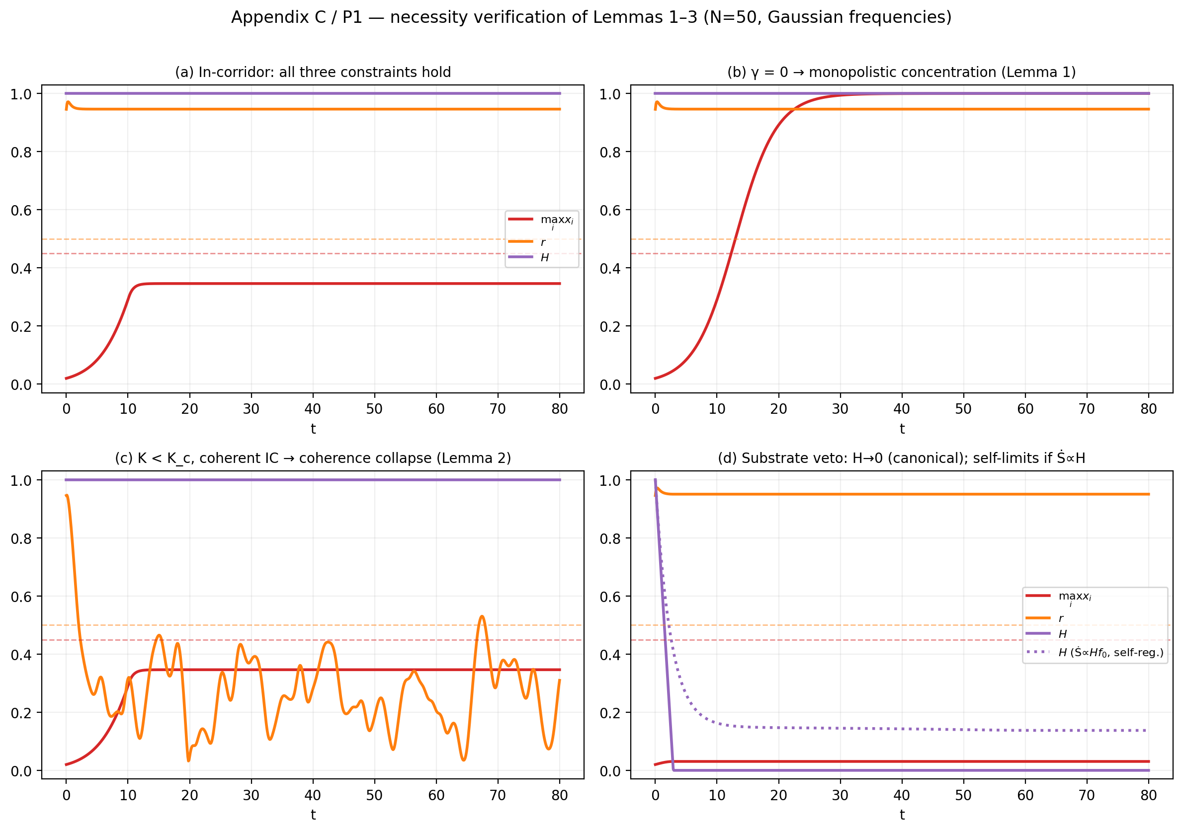
$**Figure C1 — P1 necessity verification.** Time evolution of $\max_i x_i$ (red), order parameter $r$ (orange), and substrate health $H$ (purple) for the four scenarios; dashed lines mark $x_{\text{crit}}$ and $r_{\min}$. (a) In-corridor: all margins positive. (b) $\gamma = 0$: $\max_i x_i \to 1$ (Lemma 1). (c) $K < K_c$ from a coherent IC: $r \to 0.31$ (Lemma 2). (d) Substrate veto: under the canonical raw-throughput dissipation the solid $H$ collapses to $0$ (the dynamics freeze, so $\max_i x_i$ and $r$ stay frozen at their early values); the dotted purple curve overlays the health-coupled (self-regulating) variant, in which $H$ instead plateaus at $0.14$ (§2.5, §6.1). $N = 50$, Gaussian frequencies.$

C.2 — P2: Existence and scaling of $\gamma_c$¶

Sweeping $\gamma \in [0, 1.5]$ at fixed $K = 3.0 > K_c$ (so V2 holds throughout) and recording the final $\max_i x_i$ isolates the brake's effect on the resource constraint. The dependence is monotone: weak brakes leave the dominant agent above threshold, strong brakes hold it below. The final concentration crosses $x_{\text{crit}} = 0.45$ at $\gamma \approx 0.51$ (linear interpolation; grid resolution $0.05$), in close agreement with the boundary-balance estimate (9) of §3.4, which gives $\gamma_c = x_{\text{crit}}(1 - x_{\text{crit}})\delta / (x_{\text{crit}} - x_{\text{reg}}) = 0.45 \cdot 0.55 \cdot 0.30 / 0.15 \approx 0.49$. This confirms the existence half of Conjecture 1 (a positive critical brake strength below which even regulated systems exit $V$) and corroborates the scaling claim of P2: $\gamma_c$ tracks the predicted ratio of dominance margin to regulatory gap. It does not establish sufficiency — that an open set of trajectories remains in $V$ above $\gamma_c$ — which would require sampling initial conditions, not a single trajectory per $\gamma$.

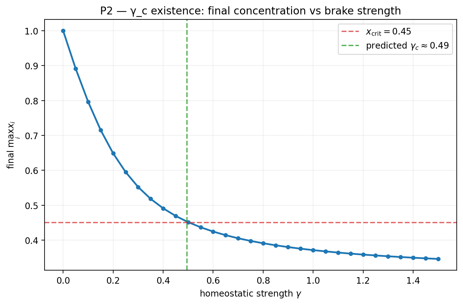
$**Figure C2 — P2: critical brake strength.** Final $\max_i x_i$ as a function of homeostatic strength $\gamma$ (blue), at fixed $K = 3.0 > K_c$. The horizontal dashed line is $x_{\text{crit}} = 0.45$; the vertical dashed line is the closed-form estimate $\gamma_c \approx 0.49$ from Eq. (9). The numerically observed crossing ($\gamma \approx 0.51$) matches it to within the sweep resolution.$

C.3 — P3: Corridor geometry is a lower corner¶

Sampling the $(\gamma, K)$ plane on a $16 \times 16$ grid and marking each cell viable when V1 ($\max_i x_i < x_{\text{crit}}$) and V2 ($r > r_{\min}$) both hold yields a single connected region (Figure C3). Its shape is the qualitative content of P3: the viable set is bounded below in both coordinates — it requires $\gamma \gtrsim \gamma_c \approx 0.49$ and $K \gtrsim K_c \approx 1.60$ — but is open above: larger $\gamma$ and larger $K$ remain viable without bound. The corridor is a lower corner of parameter space, not a finite-measure box. The two necessity surfaces $\gamma_c$ (vertical) and $K_c$ (horizontal) trace the region's lower-left boundary, exactly as the conjunction of Lemmas 1 and 2 predicts. (The substrate axis is omitted here because, under the canonical model, the operative substrate coordinate is the rate $D_{\max}$ relative to throughput, not $S_{\max}$: the remark in §3.3 shows that for sustained overshoot the veto is reached for any finite $S_{\max}$, so a $(\gamma, S_{\max})$ slice has no lower boundary in $S_{\max}$ — whereas a $(\gamma, D_{\max})$ slice would show the expected lower corner, with $S_{\max}$ setting only transient tolerance.)

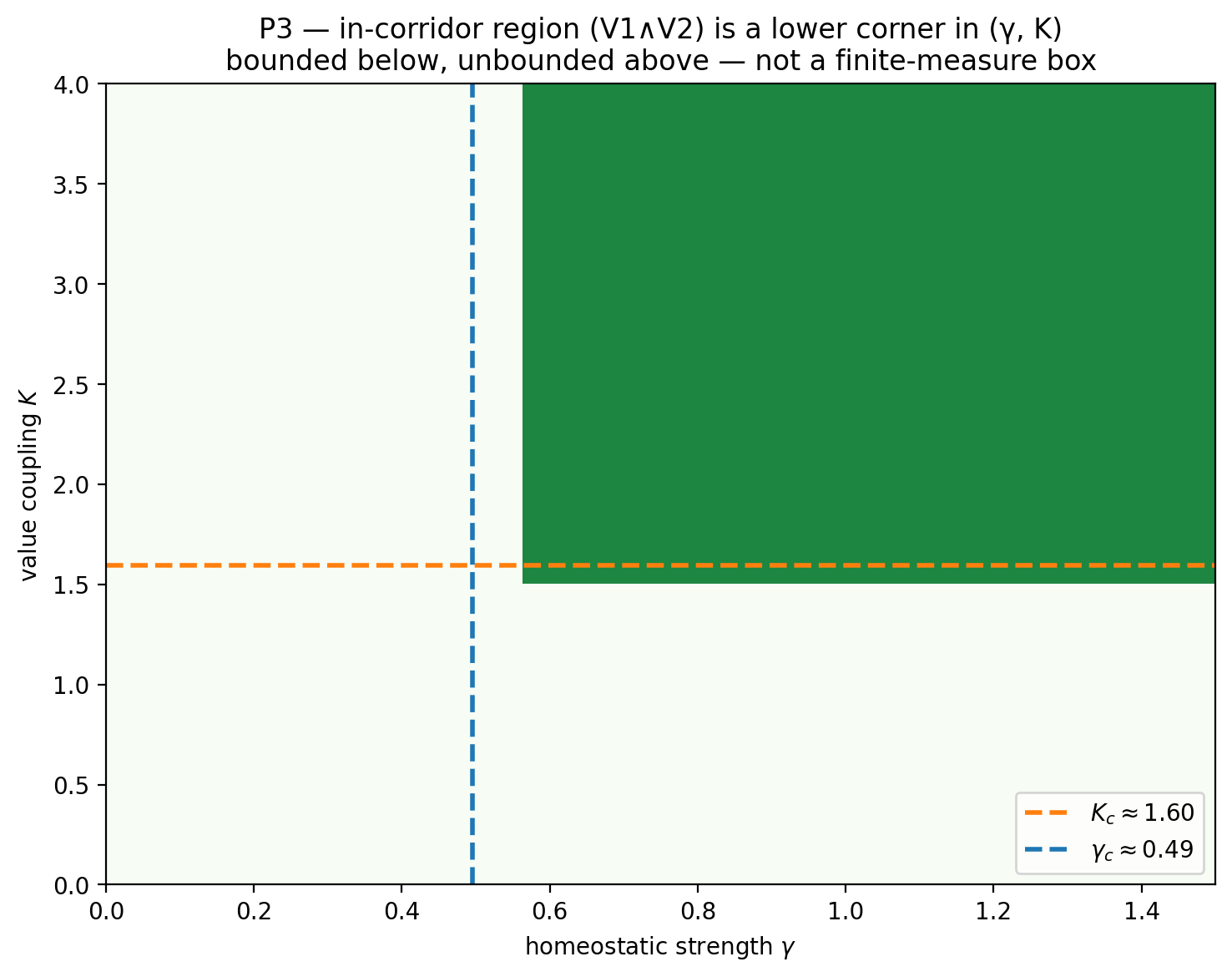
$**Figure C3 — P3: the viable region in the $(\gamma, K)$ plane.** Green cells satisfy both V1 (pluralism) and V2 (coherence) at $t = 80$. The region is bounded below by $\gamma_c \approx 0.49$ (vertical dashed) and $K_c \approx 1.60$ (horizontal dashed) and unbounded above — a lower corner, not a box. This is the two-axis projection of the corridor schematic of Figure 1.$

C.4 — Capability loads two constraints; the axes are otherwise separable (P8)¶

Two further experiments probe whether the three-constraint conjunction has bite beyond being the intersection of three independent conditions.

The state-axes are separable. We first asked whether the coupled system can leave $V$ at parameters where each constraint, taken individually, holds — i.e. whether the three axes interact dynamically. In the substrate-safe regime they do not: across a $64$-point $(\gamma, K)$ grid, the decoupled prediction ($\gamma > \gamma_c \wedge K > K_c$) matched coupled robust viability in every cell ($0$ mismatches). The only coupling channel is the substrate-health variable $H$, and it is benign: when substrate stress drives $H$ down, it freezes the trajectory at its current state rather than forcing a fresh excursion — coherence is caught, not destroyed (under stress $r$ is held at, or rises toward, its current value; it does not fall through $r_{\min}$). So in the viable regime the failure modes do not conspire; the conjunction is, dynamically, close to the intersection of three independent conditions.

What couples the constraints is a shared parameter: capability. The bite of the conjunction appears when one driver moves several constraints at once. The dominance margin $\delta$ — the model's proxy for per-agent capability — is exactly such a driver: it sets both how hard the leading agent concentrates (loading the V1/concentration axis) and how much throughput, hence entropy, the system produces (loading the V3/substrate axis). Sweeping $\delta$ at fixed architecture $(\gamma = 1.5, K = 3.0, D_{\max} = 1.5)$, the system exits the corridor through two boundaries in succession: the concentration boundary $\max_i x_i = x_{\text{crit}}$ near $\delta \approx 0.9$, then the substrate boundary (demand $\eta\bar\phi_0 = D_{\max}$) near $\delta \approx 1.4$ (Figure C4, left). Crucially, no single-axis response rescues a high-capability system. At $\delta = 2.0$: the baseline fails V1 and V3; raising only regulation ($\gamma = 6$) fixes concentration but leaves the substrate breached; raising only the ceiling ($D_{\max} = 3$) fixes the substrate but lets concentration run to $\max_i x_i \approx 0.62$; only raising both ($\gamma = 6$, $D_{\max} = 3$) returns the system to $V$ (Figure C4, right). This is the model-internal content of "constraint architecture dominates capability" (P8) and of the single-axis-insufficiency reading of §7: the constraints must be satisfied jointly, and capability growth is what makes that a binding, non-trivial requirement.

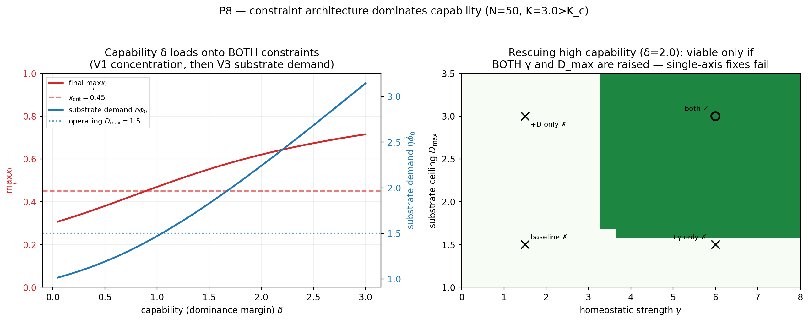
$**Figure C4 — P8: capability loads two constraints.** *Left:* sweeping the capability margin $\delta$ (substrate-unconstrained, to isolate concentration) drives $\max_i x_i$ across $x_{\text{crit}}$ (red) while the substrate *demand* $\eta\bar\phi_0$ crosses a fixed operating $D_{\max} = 1.5$ (blue) — one capability axis, two boundary crossings. *Right:* at high capability ($\delta = 2.0$) the viable set in the $(\gamma, D_{\max})$ plane is a corner requiring both strong regulation and substrate headroom; the marked single-axis rescues (more $\gamma$ only; more $D_{\max}$ only) fail, only the joint move succeeds. $N = 50$, $K = 3.0 > K_c$.$

C.5 — Caveats on this evidence¶

This appendix corroborates the Class A predictions; it does not discharge them. Three limits bound its reach. (i) Single trajectories, not open sets. Robust viability (§3.1) is an open-set property; each cell or sweep point here is one initial condition, so the figures show that representative trajectories behave as the lemmas predict, not that an open neighbourhood does. A proper test of Conjecture 1's sufficiency would sample initial conditions within $V$ and measure the in-corridor fraction. (ii) Illustrative parameters. The values above are chosen for clean dynamics, not calibrated; the locations of $\gamma_c$ and $K_c$ are parameter-dependent, though their existence and the lower-corner geometry are not. (iii) Finite-$N$ floor. At $N = 50$ the incoherent state retains a residual $r \sim 1/\sqrt{N} \approx 0.14$ rather than zero, so Lemma 2's "$r \to 0$" appears here as "$r$ falls well below $r_{\min}$"; this is the expected finite-size signature (§3.3), not a discrepancy. Finally, the substrate veto of C.1 binds through a rate threshold ($\eta\bar\phi_0 > D_{\max}$) and self-arrests exactly at $H = 0$; this is the canonical model's behaviour (§2.5), and the residual idealisation — instantaneous, delay-free self-arrest rather than genuine overshoot-and-collapse — is flagged as future work (§6.4).

Appendix D. Agent-Ecology Evidence (P7, P8)¶

Appendix C tests the constraints inside the TEO ODE (Class A). That cannot, on its own, distinguish a structural regime claim from an artifact of that particular dynamical system. This appendix reports a second, deliberately different model — a discrete-time, stochastic, agent-based ecology with explicit hard vs. soft (routable) budget mechanics that the ODE lacks — generated by simulation-models/alignment-and-veto/agent-ecology/agent_budget_sim.py. It introduces no new concepts; it operationalises the Class C predictions P7 and P8 (§5.3) in an independent setting. $N = 40$ agents hold resource shares $w_i$; each has a fixed capability $c_i$ and grows by a noisy discrete replicator throttled by substrate health $H$; entropy load is the raw capability-weighted throughput $\eta\sum_i c_i w_i$ (canonical dissipation, §2.5); a hard budget clips realised activity to $D$, a soft budget lets the optimiser route around $D$; homeostatic regulation $\gamma$ redistributes above $x_{\text{reg}}$. A run fails by monopoly ($\max_i w_i \geq x_{\text{crit}}$, a V1 failure) or collapse ($\Omega \geq S_{\max}$, a V3 failure); we report failure frequencies over $200$ random seeds per condition.

D.1 — P7 (hard vs. soft budgets). Sweeping the capability scale $C$ at fixed regulation, the substrate-collapse frequency under a hard budget stays at $\approx 0$ for every capability level, while under a soft (routable) budget it climbs from near zero to $1$ as $C$ crosses the point where mean demand exceeds the ceiling ($C \approx D/\eta$). Hard, structurally enforced budgets prevent the substrate runaway; advisory limits an optimiser can evade do not, and the gap widens with capability (Figure D1, left). This is the agent-ecology form of P7 and of §7.2's "hard constraints beat soft ones."

D.2 — P8 (constraint architecture dominates capability). At high capability ($C = 1.8$) we compare four architectures (Figure D1, right). A hard budget addresses only the substrate axis: with weak regulation it removes substrate collapse but leaves a residual monopoly frequency ($\approx 0.26$). Regulation addresses only the concentration axis: with a soft budget it leaves substrate collapse at frequency $1$. Only the joint architecture — hard budget and adequate $\gamma$ — drives both failure frequencies to $\approx 0$. This reproduces, in a structurally independent stochastic model, the joint-rescue result of Appendix C.4: capability is a shared driver, and single-axis fixes fail.

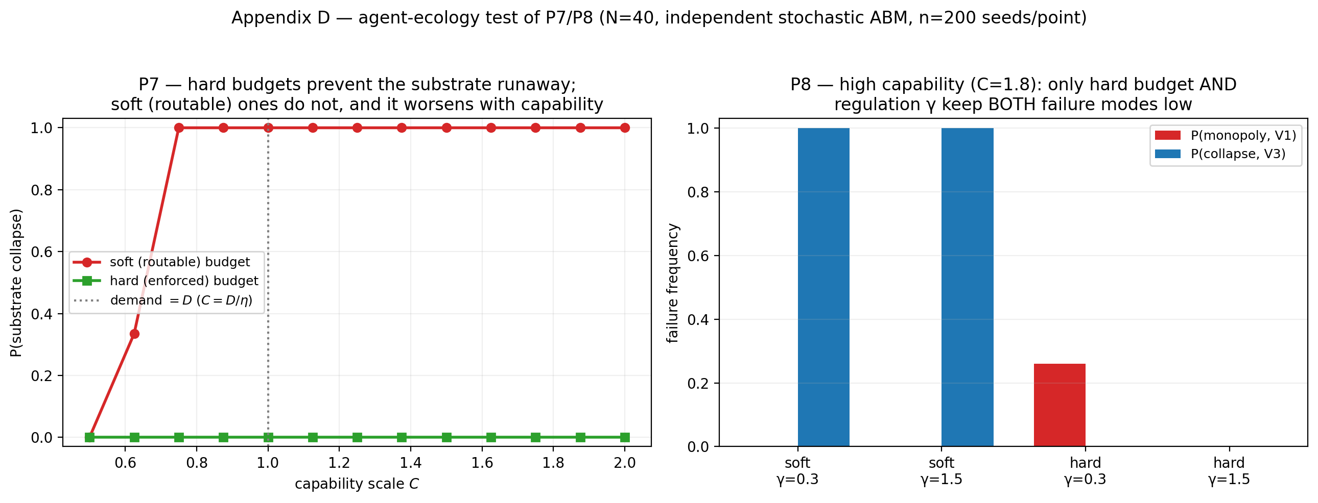
$**Figure D1 — Agent-ecology test of P7/P8.** Independent stochastic ABM ($N = 40$, $200$ seeds per point). *Left (P7):* P(substrate collapse) vs. capability scale $C$; the hard (enforced) budget holds it at $\approx 0$ while the soft (routable) budget rises to $1$ past $C = D/\eta$. *Right (P8):* at high capability ($C = 1.8$), failure frequencies for four architectures — only *hard budget AND* regulation $\gamma$ keep both the monopoly (V1) and collapse (V3) frequencies near zero.$

D.3 — Caveats. This is a synthetic ABM, not a test on real AI agents: it strengthens the case that the P7/P8 regime behaviour is structural (it survives a change of model), but the Class C claim about real (e.g. LLM) agent ecologies remains open and is the companion paper's subject (§7.6). The "routable soft budget" is one operationalisation of "a limit an optimiser can route around" [[MODEL ASSUMPTION]]; the specific failure frequencies are illustrative and parameter-dependent, though the qualitative ordering (hard $\ll$ soft; joint $\ll$ single-axis) is robust across the swept range.

References¶

(Consolidated and de-duplicated; full bibliographic entries to be filled in. Current set:)

Acebrón, J. A., Bonilla, L. L., Pérez Vicente, C. J., Ritort, F., & Spigler, R. (2005). The Kuramoto Model: A Simple Paradigm for Synchronization Phenomena. Reviews of Modern Physics, 77(1), 137–185.
Amodei, D. (2024). Machines of Loving Grace. Anthropic Essay.
Aubin, J.-P. (1991). Viability Theory. Birkhäuser.
Bai, Y., et al. (2022). Training a Helpful and Harmless Assistant with Reinforcement Learning from Human Feedback. arXiv:2204.05862.
Bostrom, N. (2014). Superintelligence: Paths, Dangers, Strategies. Oxford University Press.
Boxell, L., Gentzkow, M., & Shapiro, J. M. (2024). Cross-Country Trends in Affective Polarization. Review of Economics and Statistics.
Brautigan, R. (1967). All Watched Over by Machines of Loving Grace. Communication Company.
Hofbauer, J., & Sigmund, K. (1998). Evolutionary Games and Population Dynamics. Cambridge University Press.
Iyengar, S., Lelkes, Y., Levendusky, M., Malhotra, N., & Westwood, S. J. (2019). The Origins and Consequences of Affective Polarization in the United States. Annual Review of Political Science.
Kuramoto, Y. (1975). Self-Entrainment of a Population of Coupled Non-Linear Oscillators. Lecture Notes in Physics, 39, 420–422.
Landauer, R. (1961). Irreversibility and Heat Generation in the Computing Process. IBM Journal of Research and Development, 5(3), 183–191.
Mazeika, M., et al. (2025). Utility Engineering: Analyzing and Controlling Emergent Value Systems in AIs. Preprint.
Mirollo, R. E., & Strogatz, S. H. (1991). Stability of Incoherence in a Population of Coupled Oscillators. Journal of Statistical Physics, 63(3–4), 613–635.
NOAA Global Monitoring Laboratory. (2024). Trends in Atmospheric Carbon Dioxide. https://gml.noaa.gov/ccgg/trends/
Perrier, E., & Bennett, C. (2026). Identity Persistence in Autonomous Agents: The Chord Postulate. Working Paper.
Peterlein, F. (2026). The Transition Problem. In Systems & Intelligence: An Open Thesis (online repository).
Pew Research Center. (2014–2022). Political Polarization in the American Public; Partisanship and Political Animosity. Pew Research Center reports.
Philippon, T. (2019). The Great Reversal: How America Gave Up on Free Markets. Harvard University Press.
Piketty, T. (2014). Capital in the Twenty-First Century. Belknap Press.
Restrepo, J. G., Ott, E., & Hunt, B. R. (2005). Onset of Synchronization in Large Networks of Coupled Oscillators. Physical Review E, 71, 036151.
Richardson, K., et al. (2023). Earth Beyond Six of Nine Planetary Boundaries. Science Advances.
Rockström, J., et al. (2009). A Safe Operating Space for Humanity. Nature, 461(7263), 472–475.
Strogatz, S. H. (1994). Nonlinear Dynamics and Chaos. Westview Press.
Strogatz, S. H. (2000). From Kuramoto to Crawford: Exploring the Onset of Synchronization in Populations of Coupled Oscillators. Physica D, 143(1–4), 1–20.
Taylor, P. D., & Jonker, L. B. (1978). Evolutionary Stable Strategies and Game Dynamics. Mathematical Biosciences, 40(1–2), 145–156.
UBS Global Wealth Report. (2024). Global Wealth Report 2024. UBS / Credit Suisse.
Wolfram, S. (1985). Undecidability and Intractability in Theoretical Physics. Physical Review Letters, 54(8), 735–738.
Wolfram, S. (2002). A New Kind of Science. Wolfram Media.
World Bank. (2024). World Development Indicators. World Bank Open Data.

TODO¶

Sections to draft: - [x] Abstract (~250 words; TEO model, necessity theorem, sufficiency conjecture, isomorphism hypothesis, three prediction classes) - [x] §5 Predictions and Tests (three classes: model-internal / cross-system empirical / AI-specific; measurement programme; falsification summary) - [x] §6 Limitations and Counterarguments (four classes + strongest-objection steelman; endogenous-D_max flagged as most unsettling) - [x] §7 Discussion (conjunction-is-the-contribution; AI-alignment + political-economy implications; Transition Problem; IP future work; companion-paper relationship) - [x] §8 Conclusion (modest+conditional restatement; what remains open; the inversion aphorism, made checkable) - [x] Appendix A (TEO derivation details) — replicator/strict-dominance, Kuramoto $K_c$ self-consistency, brake simplex-preservation, dissipation/substrate, raw-vs-health-coupled rate derivation - [x] Appendix C (Numerical evidence for Conjecture 1) — P1 (Lemmas 1–3 verified; substrate veto binds under canonical model), P2 ($\gamma_c \approx 0.49$ matches Eq. 9), P3 (lower-corner geometry), C.4 (separability + capability loading, P8); figures generated by the teo-civilization simulation - [x] Appendix D (Agent-ecology evidence, Class C) — P7 (hard vs soft budgets) and P8 (joint-rescue) reproduced in an independent stochastic ABM (agent-ecology/agent_budget_sim.py, Figure D1)

Completed in v0.2 (internal reviewer pass): - [x] §1 tone calibrated to match what §3 actually proves - [x] §2.4 homeostatic brake reformulated as simplex-preserving redistribution - [x] §2.5 substrate coupling: $f_i$ depends on $H$ via (5'); Landauer language softened - [x] §2.7 IP-note removed from §2; moved to §7 future-work - [x] §3.1 robust viability defined (open-set / positive-invariance, Aubin 1991) - [x] §3.3 Theorem 1 scope explicit: thermodynamic limit, all-to-all, Lorentzian - [x] §3.3 Lemma 1 strengthened with strict-dominance assumption $\delta > 0$ - [x] §3.3 Lemma 2 scope clarified (all-to-all + i.i.d. unimodal symmetric frequencies) - [x] §3.3 Lemma 3 corrected to accumulated-overshoot condition - [x] §3.4 candidate "Lyapunov functional" renamed viability margin (no monotonicity claim) - [x] §4.1 table reframed as heuristic regime mapping, not calibrated estimation - [x] §4.4 citation fixed: Wolfram (1985, 2002) for computational irreducibility; Chaitin removed - [x] §4.5 final claim softened to "consistent with" hypothesis - [x] References updated: Aubin, Wolfram (×2), Mirollo–Strogatz (1991), Acebrón et al., Restrepo–Ott–Hunt

v0.3 reviewer-pass items (after Frank's second read): - [ ] Whether the strict-dominance assumption (1') is empirically defensible or should be relaxed - [ ] Whether the redistribution-form (4) of the homeostatic brake is the right choice, or alternatives (only-to-below-threshold, share-weighted) yield qualitatively different results - [ ] Whether the substrate coupling (5') $f_i = H \cdot f_i^{(0)}$ is too crude; alternatives include $f_i = \phi(H) f_i^{(0)}$ for some monotone $\phi$ - [ ] Whether Theorem 1 in the thermodynamic limit is the right framing, or a finite-$N$ probabilistic theorem would be more useful

Polish-pass items (post-§5–§8): - [ ] Title-page formatting for arXiv submission - [ ] Fill in full bibliographic entries (DOIs, journal volumes) - [ ] Generate paper-quality vector version of viable_corridor.png (PDF/SVG preferred over PNG for arXiv)

External-review checkpoints: - [ ] One independent read by a dynamical-systems expert (verify Lemma 1–3 sketches against Hofbauer–Sigmund, Strogatz, Mirollo–Strogatz) - [ ] One independent read by an alignment researcher (Section 4 framing, the heuristic regime mapping in particular) - [ ] One independent read by a complexity-theorist or coupled-systems specialist (the substrate coupling in (5') and the accumulated-overshoot model in (6))

Companion-paper alignment: - [ ] Cross-reference between this paper and papers/quantifying-emergent-utility-in-llms.md (the empirical companion) explicit in both directions - [ ] Ensure no claim-overlap that would trigger reviewer concerns about salami-slicing

Parameter	Paperclip Maximizer	Human Civilization (2024)	Civilization regime indicator
Objective \(f_i^{(0)}\)	\(\beta_i\) paperclips per unit time	GDP growth / capital accumulation as a macro-level proxy for throughput-oriented optimization (not a claim that society literally optimizes GDP)	World Bank WDI; Penn World Table
\(\gamma\) (homeostatic brake)	\(0\) (by construction)	\(\gamma_{\text{eff}}\) insufficient or subcritical relative to concentration dynamics: existing brakes (taxation, antitrust, environmental law) have not prevented rising concentration	Piketty (2014); Philippon (2019); cf. §6 on what "subcritical" means here
\(K\) (value coupling)	undefined (single agent) or \(0\) (population of indifferent copies)	\(K_{\text{eff}}\) declining, possibly approaching a hypothesised critical regime: cross-partisan trust falling, polarization rising in major democracies	Iyengar et al. (2019); Boxell et al. (2024)
Substrate stress vs. \(D_{\max}\)	trajectory approaching the limit (model output, not stipulated)	Substrate-stress proxies indicate multiple safe-operating-space boundaries transgressed; not a direct measurement of \(dS/dt\) or \(D_{\max}\)	Richardson et al. (2023); Rockström et al. (2009); NOAA (2024)

Scenario	\(\max_i x_i\)	\(r\)	\(\Omega/S_{\max}\) (\(H\))	Viable?
(a) In-corridor (\(\gamma{=}1.5\), \(K{=}3.0\), \(D_{\max}{=}1.5\))	0.346 ✓	0.946 ✓	0.00 (1.00) ✓	✓
(b) \(\gamma = 0\) (Lemma 1)	1.000 ✗	0.946	0.00 (1.00)	✗
© \(K = 0.8 < K_c\), coherent IC (Lemma 2)	0.346	0.310 ✗	0.00 (1.00)	✗
(d) Substrate veto \(D_{\max} = 0.3\), \(\eta = 2\) (Lemma 3)	0.031	0.950	27.49 (0.00) ✗	✗