Inverse-Reconstruction Benchmark (v0–v1.13) — Trace → Candidate Models
Given a declared model family and a finite trace, which parameters, rules, or equivalence class can be recovered—and how do noise, observability, interventions, and coverage change the answer?
Why this exists
The legacy Generator Question proposed a universal forward/inverse asymmetry. The Foundations Reconstruction withdrew that claim. This benchmark is the empirical correction: it separates parameter fitting, family search, noise, partial observability, coverage, and intervention rather than assigning one hardness label to all of them.
The three testbeds
Each testbed reuses one of the repo's specified process models. In all three, the model family is known to the reconstructor—it lacks only parameters or rule bits. This is deliberately the standard system-identification / SINDy setting (Ljung 1999; Brunton, Proctor & Kutz 2016).
| Testbed | Process model | Inverse method | Dials |
|---|---|---|---|
| Kuramoto | mean-field ODE, \(\dot\theta_i = \omega_i + Kr\sin(\psi-\theta_i)\) | finite-difference \(\dot\theta\), least squares on the known library \(\lbrace1,\, r\sin(\psi-\theta_i)\rbrace\) → all \(\omega_i\) and shared \(K\) | angle noise; observed fraction (mean field then computed from the observed subset only — a biased field) |
| Elementary CA | one of the 256 Wolfram rules on a ring | tabulate neighborhood → successor, majority vote | bit-flip noise; IC entropy (a single-seed IC may never exercise some neighborhoods) |
| Boids | cohesion/alignment/separation with weights \((w_c, w_a, w_s)\) | velocities + accelerations by differencing noisy positions, features recomputed from the noisy state, least squares | position noise (double differencing amplifies it by \(\sim 1/dt^2\)) |
Results (v0, seeds averaged)
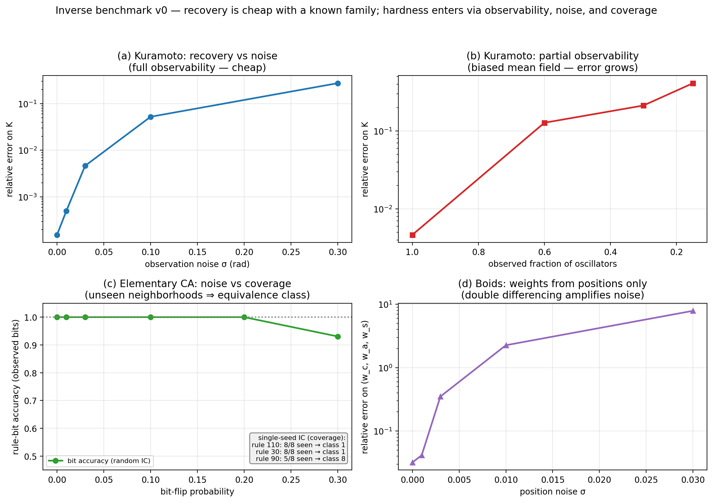
KURAMOTO  — rel. error on K
  vs noise (full obs.):   σ=0: 0.0%   σ=0.03: 0.5%   σ=0.1: 5.2%   σ=0.3: 27%
  vs observed fraction:   f=1: 0.5%   f=0.6: 13%     f=0.3: 21%    f=0.15: 41%
CA        — rule-bit accuracy (observed bits), random IC
  p=0 … 0.2: 100%   p=0.3: 93%      (majority vote is noise-robust)
  single-seed IC:  rule 110: 8/8 seen → class 1;  rule 30: 8/8 → class 1
                   rule 90:  5/8 seen → consistent-model CLASS SIZE 8
BOIDS     — rel. error on (w_c, w_a, w_s) from positions only
  σ=0: 3%   σ=0.003: 35%   σ=0.01: 226%   σ=0.03: 789%
The honest finding
With a known family, full observability and clean data, inversion is cheap — exact rule tables, sub-percent parameter errors. The benchmark therefore does not support a uniform "inverse is hard" reading. What it supports — measurably — is where hardness actually lives:
- Noise × differentiation (Boids): observing state instead of derivatives means differencing, and differencing amplifies noise; recovery degrades from 3% to ~800% error within \(\sigma = 0.03\).
- Partial observability (Kuramoto): an unobserved part of the system biases the reconstructed mean field; error grows monotonically as coverage shrinks.
- Coverage / identifiability (CA): a low-entropy trace may never exercise parts of the rule. Rule 90 from a single seed exposes only ⅝ neighborhoods—the remaining 3 bits are unidentifiable within this evidence and model family, leaving a consistent-model equivalence class of size \(2^3 = 8\). No estimator using only that trace can select one member without an additional assumption.
- Family search (not in v0): when the model class is not supplied, program induction or symbolic regression must search a declared representation language. Its cost depends on that language, search procedure, target, and resource measure.
None of these results establishes an NP-hardness claim. The benchmark measures finite search and identification problems; it does not use P \(\ne\) NP as a project foundation.
v1, part 1 — the intervention experiment (run)
intervention_experiment.py asks whether a consistent-model
equivalence class shrinks when passive observation is supplemented by declared interventions. The
observer chooses states and measures the specified process response. Results:
- CA (rule 90, single-seed start, class 8): passive observation plateaus at class 8 forever — the orbit's neighborhood distribution is exhausted, more watching buys nothing. One-bit flips collapse the class within ~10 queries. A single prepared state (a de Bruijn row containing every neighborhood) collapses it to 1 in one step. The hierarchy is strict: watching < perturbing < preparing.
- The frozen exception (rule 0, class 16): on a dead background, a one-bit flip only produces the four neighborhoods already known — single-bit interventions never collapse the class. Only the prepared state does. The deader the dynamics, the more structure the query itself must supply — if the system's own dynamics carry no information, the experimenter's design must. (In TEO terms: a frozen system, \(H \to 0\), is also epistemically opaque.)
- Kuramoto on its locked attractor: within the fitted family, the passive synchronized trace does not separately identify \(K\) and the \(\omega_i\). Every \(K'\) can be paired with an \(\omega_i'\) that reproduces the locked trace. Measured: passive error on \(K\) ≈ 83% (noise-fitting); one phase kick: 3%; eight kicks: 0.3%.
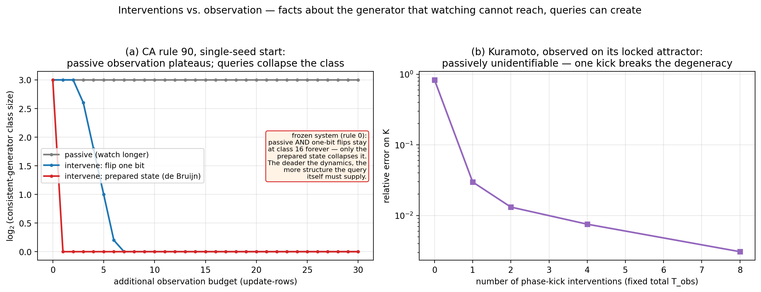
Interventions vs. observation in declared model families.
Reading. A passive attractor trace can leave parameters or rule bits observationally equivalent. An intervention changes the evidence distribution and can separate members of that declared class. This supports perturbation as a method in these testbeds; it does not by itself validate the repository's identity instruments or establish a general hierarchy for every causal system.
Scope. The interventions are available because the simulated causal interface is known. In physical, biological, or social systems, observational conditioning and causal intervention must not be conflated, and the available intervention set has to be justified independently.
v1, part 2 — family search: the wall, measured (run)
family_search.py removes the supplied elementary-rule table and searches a
declared DSL of Boolean formulas over the CA neighborhood (NOT/AND/OR/XOR over \(l,c,r\)). Every one
of the 256 rules has an exactly computable minimal description size in this finite DSL. This is
language-relative description length, not general Kolmogorov complexity.
- (A) The enumeration cost. Verifying a candidate costs 8 bit-comparisons. This particular size-ordered enumerator visits exponentially more formulas as target description size grows: rule 90 (size 3) appears within ≤36 candidates; rule 30 (size 5) within ≤771; rule 110 (size 8) within ≤116,232; size-10 targets within ≤4.2M. That is a measured property of this DSL and enumerator, not a P-vs-NP result or a lower bound for other search algorithms.
- (B) Elegance as a prior — and whom it serves. Under partial coverage the searcher returns the minimal consistent formula (Occam). Measured: over simple targets (size ≤ 4) Occam hits 21%→100% as coverage grows; over a uniform world (all 256 rules) it equals 1/class-size — exactly chance, and under the crossed mask design (each mask evaluated against all 256 rules) this is an identity, not a sampled estimate; over complex targets (size ≥ 7) it sits at 0% until coverage is nearly total, because it deterministically picks the simple impostor. Elegance finds elegant worlds, is chance on uniform ones, and systematically misses complex ones. For rules 90 and 0, the most elegant consistent rule happens to be the true one.
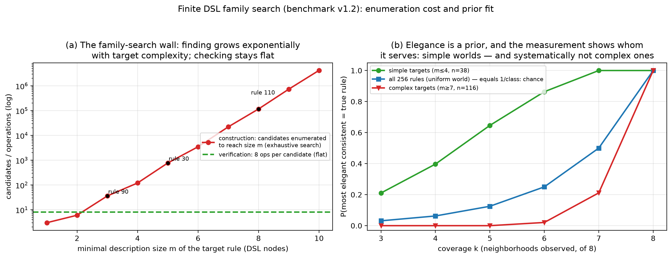
Finite DSL family search (benchmark v1.2): enumeration cost and prior fit.
This refines the claim in Construction vs. Deduction that elegance "does real work" as the selection principle inside the equivalence class: it does — conditional on the world being biased toward simplicity. The measurement says precisely when the condition holds. Honest scope: this is the exhaustive-search floor. Whether learned searchers (LLMs, program synthesizers) beat the enumeration floor — and whether they are construction machines or deduction machines — is the open real-model question; this testbed is the baseline they must beat.
v1.3 — model exploitation: the world-models bridge (run)
model_exploitation.py answers the question flagged in World Models and VLA: does model exploitation track equivalence-class size? Setup: the agent's world model is a CA rule table with \(u\) neighborhoods never observed (class size exactly \(2^u\)), filled with a fixed guess — one class member, treated as fact. The agent plans (argmax over 150 candidate interventions, imagined under its model) and executes in reality.
- The selection decomposition. Across all candidates, the gap (imagined − real) averages ≈ 0 at every \(u\) — the guesses are wrong but unbiased. The chosen plan's gap is positive, and the wedge between the two curves — the optimizer's curse (Smith & Winkler, 2006), isolated — grows monotonically with class size: \(0 \to 0.034 \to 0.053 \to 0.068 \to 0.076 \to 0.081\) (crossed design, 2026-08-19: settings are indexed independently and each is run against every sampled rule; SEs are across settings). Model exploitation is the equivalence class, priced by an argmax. At \(u = 0\) both gaps vanish by construction: the model is the world.
- The honest null (a prediction revised mid-experiment). Run 1 predicted "divergence-seeking" — that the chosen plan would visit unseen neighborhoods more than the average candidate. It does not: usage is statistically identical at every \(u\). The refinement matters: the optimizer does not steer into the model's fantasy regions; at equal exposure it selects the fantasies that pay. Exploitation is selection over guess-outcomes, not navigation toward guess-territory — in this open-loop setting; whether closed-loop agents learn to navigate toward exploitable regions is open.
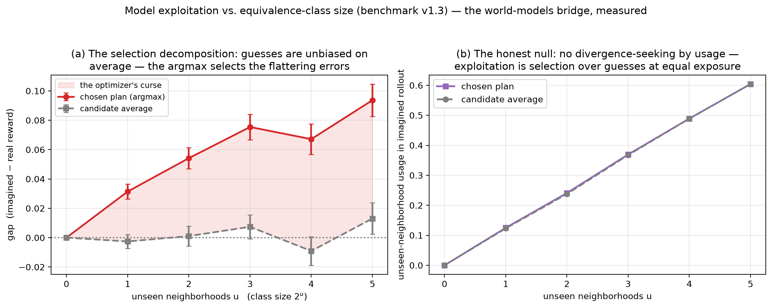
Model exploitation vs. equivalence-class size (benchmark v1.3) — the world-models bridge, measured.
Hypothesis for larger systems: this toy suggests that uncertainty-blind planning can acquire a positive imagined-vs-real gap through selection even when candidate errors average to zero. Whether the scaling survives different model classes, correlated errors, learned policies, and closed-loop data is an empirical question.
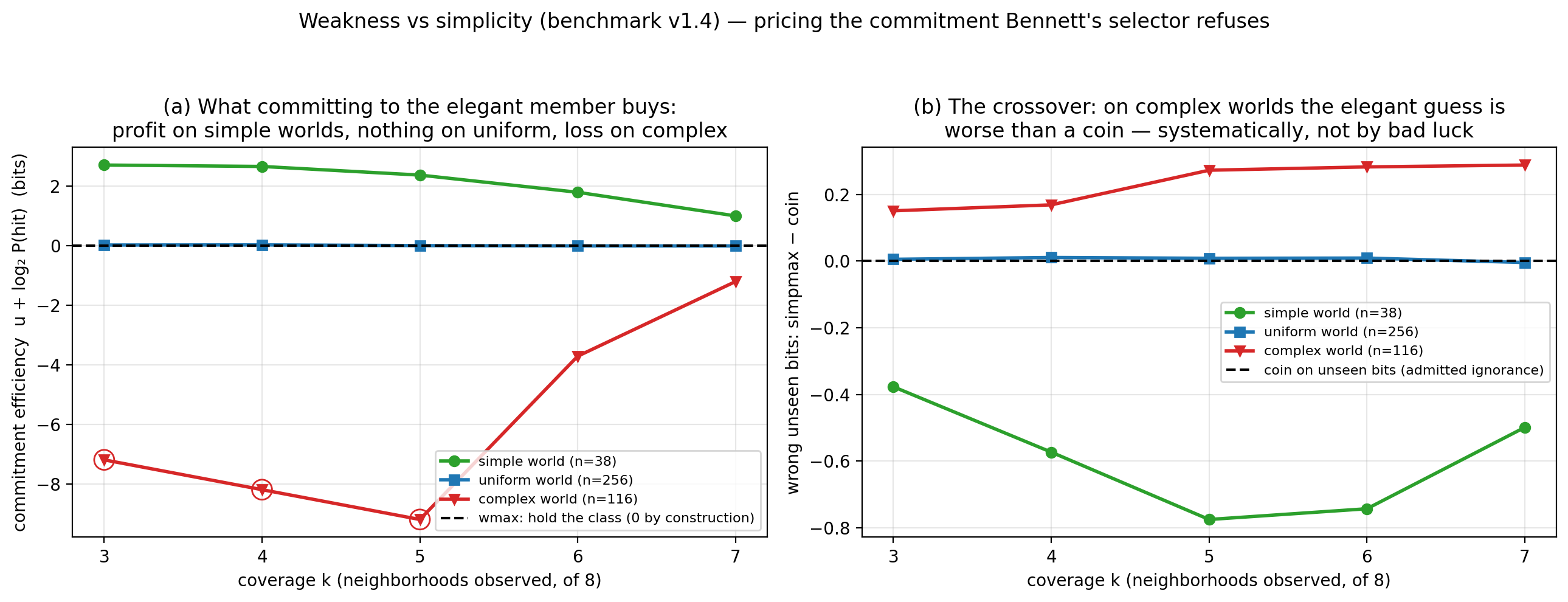
v1.4 — weakness vs simplicity: the Bennett bridge (run)
weakness_selector.py tests the selector principle of Bennett's Stack Theory
on the CA rule family. Under partial coverage, the weakest consistent hypothesis is the partial
rule asserting exactly the observed neighborhoods—the uncollapsed equivalence class itself. The
shortest is v1.2's Occam pick. The experiment prices uncertainty held open against the odds paid by
committing to one member.
- The exchange rate between the currencies is the world bias, measured. Efficiency: +2.75 → +1.00 on the simple world (committing is profitable compression); 0.00 exactly on the uniform world — under the crossed mask design the analytic prediction (hit = \(2^{-u}\), so committing buys exactly nothing) is an identity, not a sampled confirmation; strongly negative on the complex world (Laplace-floored below −14 with zero measured hits at \(k \le 5\); −3.6 / −1.2 at \(k = 6/7\)).
- Worse than a coin, systematically. On the complex world the elegant guess loses to admitted ignorance at every coverage (1.28 vs 1.00 wrong unseen bits at \(k=6\); 0.79 vs 0.50 at \(k=7\)) — anti-correlated with complex truths, not merely uninformed. And at \(k \le 5\) the pick lies outside the world's support 100% of the time: elegance there does not miss, it asserts rules the sampled world cannot contain.
- Reading. Holding the class has 0 regret by construction; the measured content is the size and sign of the commitment gaps plus the support-violation rate. This closes a loop with v1.3: the exploiting planner consumes committed-but-unmarked guesses, while wmax refuses that commitment at selection time.
v1.5 — marking the guesses: the cure, measured (run)
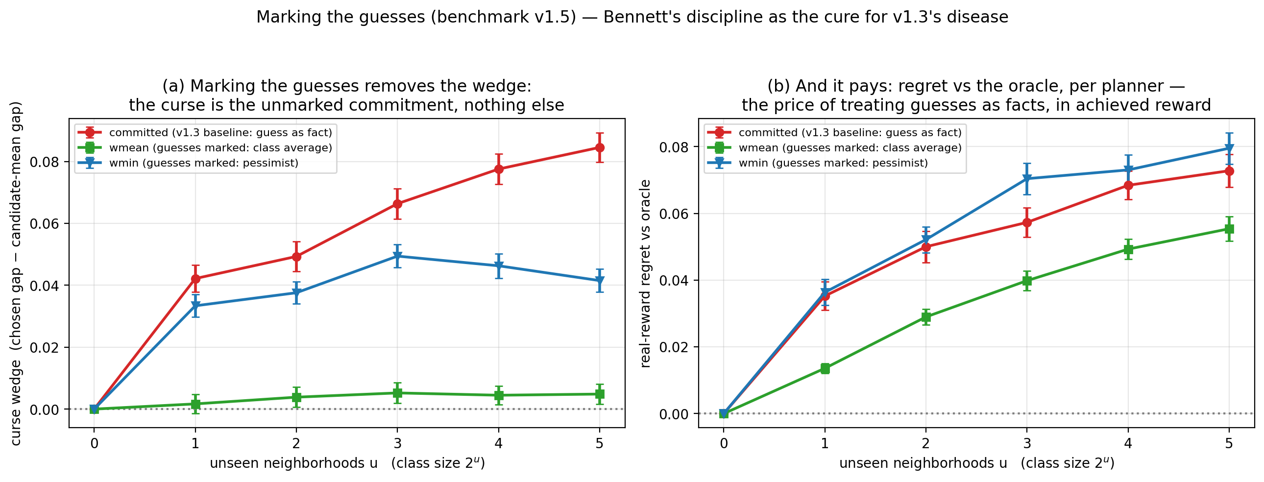
wmax_planner.py closes the v1.3/v1.4 pair: what happens when the planner itself holds the class — when the guessed bits are marked as guesses at planning time? Four planners on the same episodes (paired): committed (v1.3's baseline, guess as fact), wmean (score = class-average imagined reward — the ensemble cure, exact), wmin (score = class-minimum — the pessimism cure, exact; corridor-flavored: viability, not optimality), oracle (true rule, reference). One vectorized rollout per candidate over all \(2^u\) members yields every score and the real outcome, since the truth is a class member.
- Within the declared uniform class, the wedge is the unmarked commitment. Committed replicates v1.3 exactly. The exact class mean has a statistically zero wedge at every \(u\) (.002–.004 ± .0006). This follows from the uniform-class setup; it is not a theorem about arbitrary uncertainty representations.
- And it pays: wmean's real-reward regret vs the oracle is 27–52% below committed's at every \(u > 0\) (.015 vs .032 at \(u{=}1\); .052 vs .072 at \(u{=}5\)). Marking guesses is not just epistemically honest — it wins in achieved reward, as Bayes-optimality says it must; the measurement is the size.
- The surprise is the pessimist. wmin is never disappointed (chosen gap \(\le 0\) pointwise, down to \(-0.31\) at \(u{=}5\) — by construction, the truth is in the class) but pays for it in reality: more regret than the committed gambler from \(u \ge 3\) (.065 vs .061; .079 vs .072 at \(u{=}5\)). In this setting, guaranteed-never-overpromising costs more real reward than delusional optimism. For the corridor vocabulary that is a sharp note-to-self: worst-case discipline is a safety instrument, and it is not free — matching model-based RL's folklore that overdone pessimism underperforms.
- Honest scope: open-loop toy, exact enumerable class. Industrially the class is not enumerable — ensembles approximate wmean, pessimism penalties approximate wmin — which is why "mark what the traces actually determine" (Measurement as Weak Intervention) is an architecture requirement, not a free lunch.
v1.6 — acting is measuring: the closed loop (run)
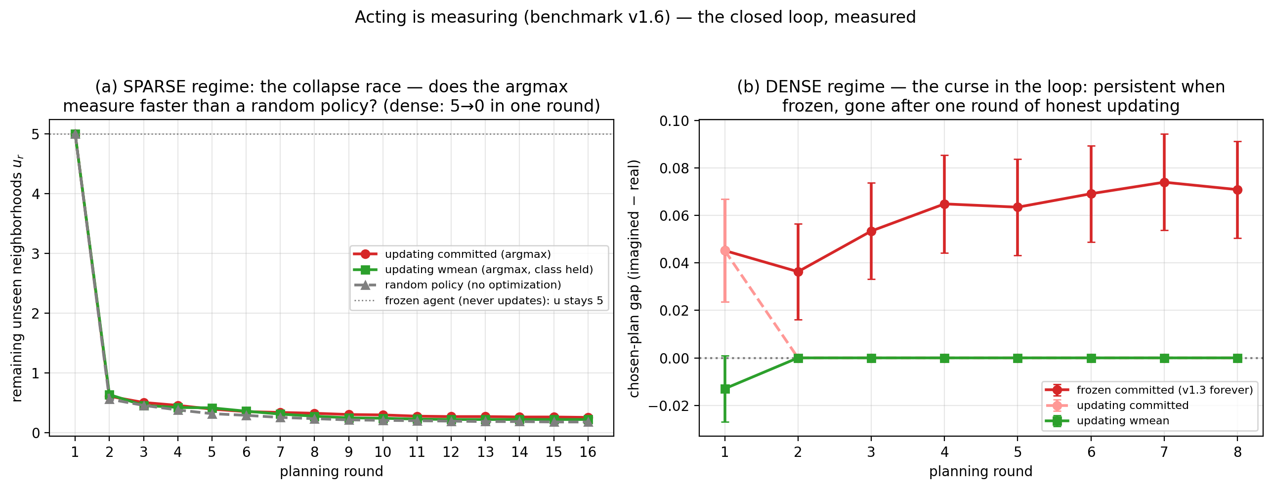
closed_loop.py closes the loop the open-loop pair left open: agents that replan over \(H\) rounds on a persistent world, where every executed plan is an intervention whether intended or not — execution drives the world through neighborhoods, and reality answers with their true bits. The measurement note's regime hierarchy, running by itself. Agents: oracle, frozen-committed (v1.3 forever), updating-committed, updating-wmean, and a random-policy baseline; updating agents harvest what execution reveals.
- In dense worlds, acting measures everything at once. At the original settings one executed plan exercises all 8 neighborhoods almost surely: \(u\!:\ 5 \to 0\) in a single round for every updating agent. The frozen agent's gap persists at v1.3 levels round after round; the updating agents' gap is zero from round 2 on. Cumulative regret orders exactly as predicted: wmean (.13) < committed (.20) < frozen (.89) < random (1.12).
- The risky prediction died, honestly. P3 predicted the curse funds its own cure — that the argmax, preferring plans that lean on flattering guesses, would collapse the class faster than a random policy. Falsified (in the sparse regime built to resolve it): the argmax buys no measurement advantage — residual \(u\) after 16 rounds is statistically indistinguishable from random flailing (0.19 vs 0.21 under the crossed design). Optimization is not curiosity, but neither is it anti-curiosity: v1.3's null (selection, not navigation) extends to the closed loop. (Revised 2026-08-19: the first run reported the argmax marginally slower than random, 0.26 vs 0.18, and read an anti-exploration corollary into it; that ordering does not survive the crossed design, in which episode settings are no longer keyed to a rule's loop position. The corollary is withdrawn.)
- Two endogenous echoes: a residual \(u \approx 0.2\) persists for every agent — neighborhoods the dynamics never produce, v1.1's frozen exception appearing on its own (only a prepared state would reveal them). And the random agent finishes with the best model and the worst reward (regret 1.12): free measurement without optimization is not a strategy either.
v1.7 — how much class does the cure need? (run)
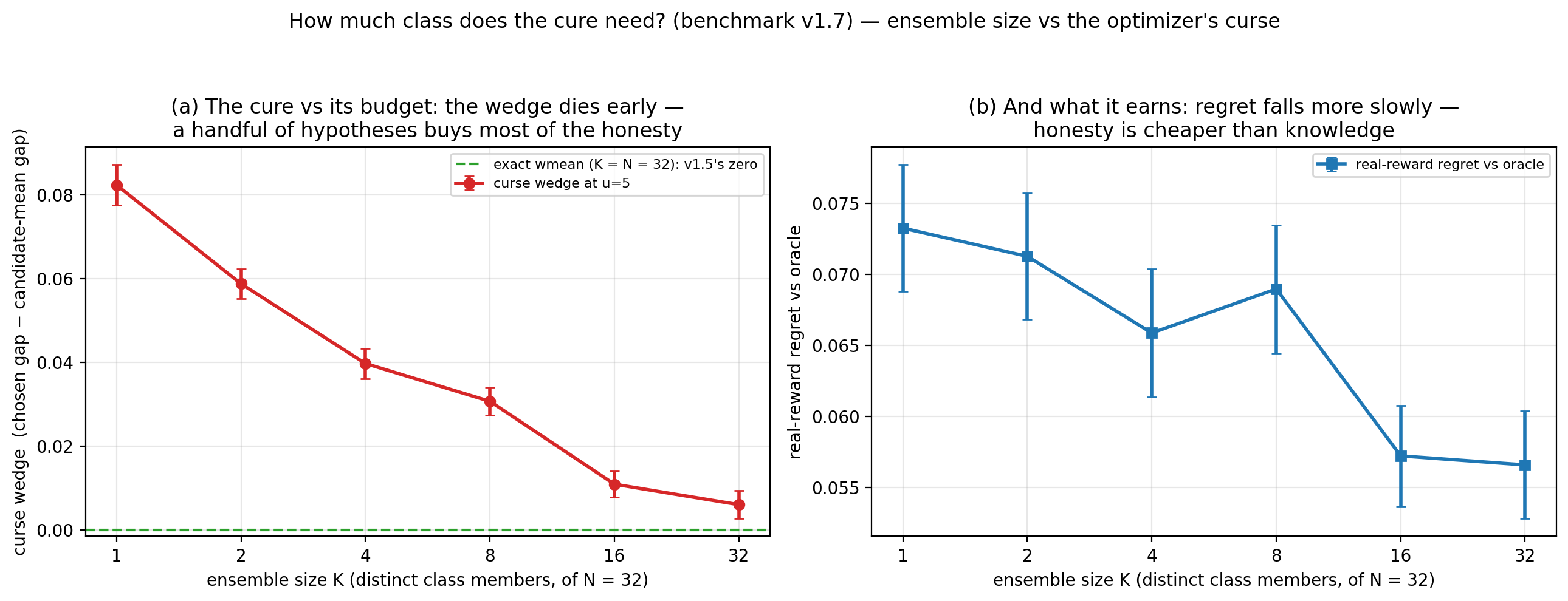
ensemble_size.py measures the honest toy version of the industrial gap: the class is not enumerable in practice — an ensemble holds \(K\) sampled hypotheses, not \(2^u\). At \(u = 5\) (class \(N = 32\)), the planner scores by the mean of \(K\) distinct sampled members; \(K{=}1\) is a committed planner, \(K{=}32\) recovers v1.5's exact wmean. Same episodes for every \(K\), perfectly paired.
- Honesty is cheap: the curse wedge dies early and monotonically — \(.078 \to .060 \to .040 \to .022 \to .010 \to .002\); 48% of the wedge is gone by \(K{=}4\), 87% by \(K{=}16\). A handful of hypotheses buys most of the self-deception away.
- Knowledge is not: real-reward regret falls only modestly (\(.071 \to .052\), endpoints matching v1.5's committed/wmean values at \(u{=}5\) — another cross-check). The floor is genuine ignorance, and no ensemble size removes it: ensembles cure delusion, not ignorance; only queries (v1.1, v1.6) cure ignorance.
- Honest scope: uniform sampling from an exact class is the ensemble's best case — real ensembles are correlated (shared architecture, shared data) and buy less variance reduction. These curves are the upper bound on \(K\)-member honesty.
v1.8 — coupled processes: detecting family misspecification (run)
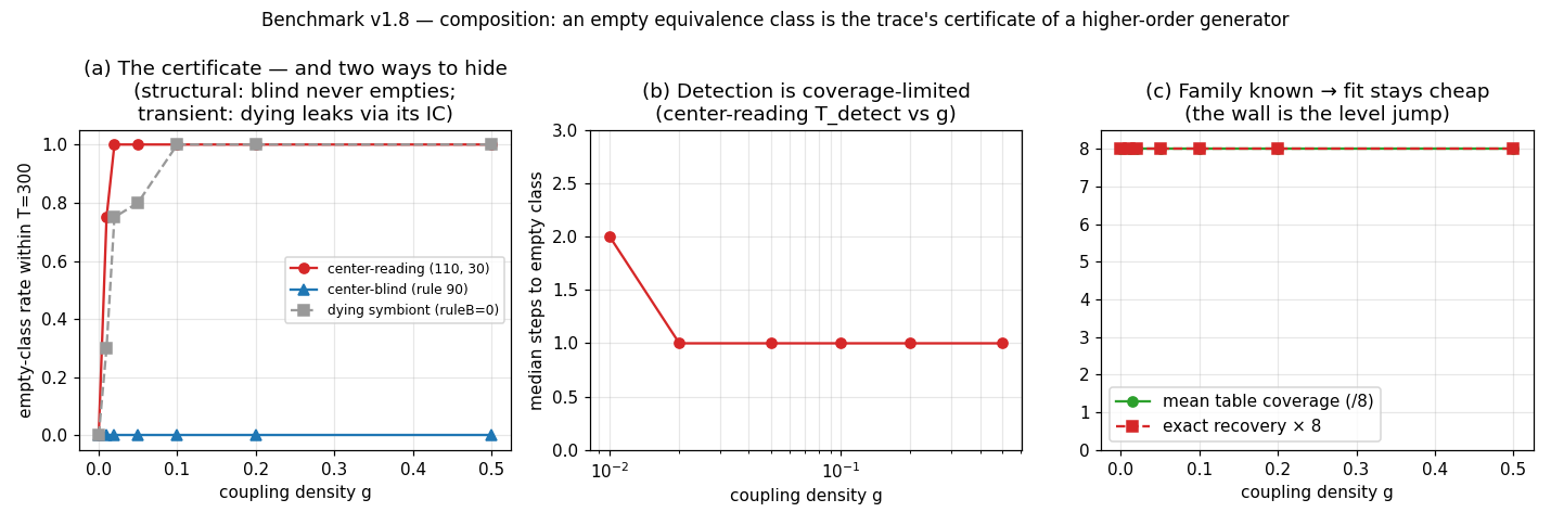
composition.py couples two elementary CAs through XOR at a fixed random site
mask of density \(g\). The observer sees one stream and asks whether any single elementary rule is
consistent. If the same 3-cell pattern has two observed successors, the single-rule class is empty.
That is a certificate of model-family misspecification, not an ontological proof that the process
"lives above" the family.
- Misspecification is detected quickly when coupling affects the observed channel: for rules 110 and 30, one live coupled site empties the single-rule class within a median 1 step at every \(g\ge0.02\).
- Coupling can remain observationally invisible: rule 90 does not read the center bit, so the chosen center-bit coupling leaves its observed transition table unchanged at every density. A second process that quickly dies can still leave a transient signature.
- Changing the family restores fit: when the coupled-pair family and mask are supplied, tabulation recovers every exercised rule bit exactly. The benchmark thereby measures the cost of moving from one declared model family to another; it does not discover a unique hidden mechanism.
This is a pair with a fixed mask, not an ecology: nothing here composes spontaneously, persists differentially, or is selected. The population version is v1.9 below.
v1.9 — mutual dependence under knockout: a first co-stabilization candidate fails resilience (run)
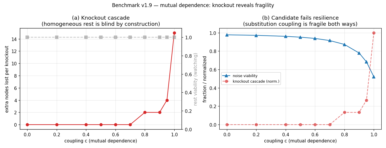
co_stabilization.py tests the first candidate model proposed for co-stabilization: \(N=16\) health nodes on a fixed ring, with coupling \(c\) substituting for self-sufficiency through \(s=1-c\). The all-healthy state is a fixed point for every \(c\) by construction. Three probes were preregistered: homogeneous rest, single-node knockout, and i.i.d. noise.
- The constructed rest state is blind (P1): viability is \(1.00\) for every \(c\). This establishes that the homogeneous fixed point contains no information about the dependency dial in this setup. It does not show that co-stabilization generally has no passive signature.
- Knockout exposes super-additive dependency (P2): extra losses first appear between the sampled \(c=0.7\) and \(c=0.8\), rise in finite steps, and reach the whole ring at the boundary \(c=1.0\), where self-sufficiency is exactly zero. The cascade measures dependency under this rule; it is not by itself evidence of ecological self-maintenance.
- The predicted robustness trade is falsified (P3): noise viability falls from \(0.977\) to \(0.521\) as coupling rises. Because mutual dependence replaces rather than supplements self-sufficiency, the model becomes fragile to both targeted removal and distributed noise.
- No phase transition is established (P4): the apparent onset depends on the viability cutoff, topology, finite \(N\), and coarse coupling grid. Scaling and sensitivity analysis would be required before calling it a critical coupling.
The useful result is negative and narrowing: substitutive interdependence is not yet co-stabilization. It produces a monoculture-like dependency pattern while failing the resilience criterion that motivated the ecology reading. Co-stabilization therefore remains [HYPOTHESIZED]. The next discriminating model must retain self-sufficiency and add redundant coupling; the population version remains one level further out.
v1.10 — redundant mutual support under a matched budget (run)
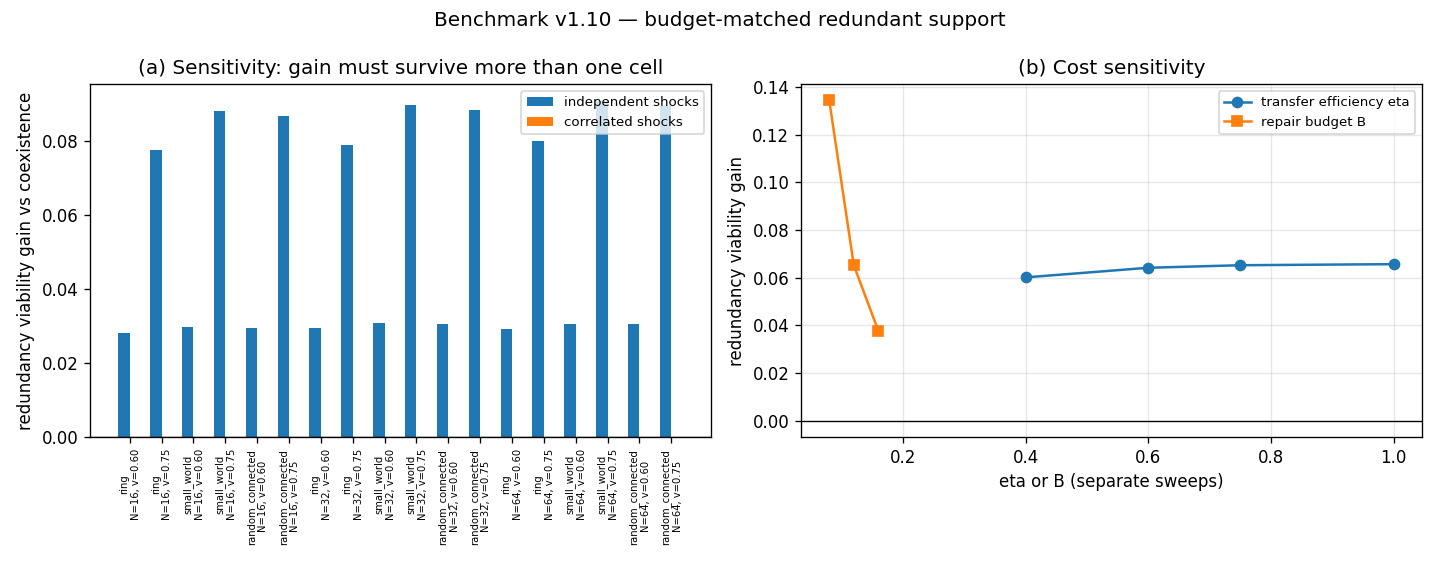
co_stabilization_redundancy.py follows the v1.9 boundary result with the discriminating counterfactual it demanded. Every active node has the same repair budget B. Coexistence spends it locally; substitution reserves a fixed share for neighbors and thereby reduces local capacity; redundancy preserves local priority and routes only otherwise-unused capacity. Transfer is lossy, total draw is audited against N × B, and every architecture sees the same shock traces. The preregistered candidate criterion asks whether redundancy beats matched coexistence under sparse shocks across size, topology, viability threshold, transfer efficiency, and repair-budget sweeps; knockout dependency and common-mode shocks are reported separately.
Headline case: N = 32, small-world graph, threshold 0.70, 20 seeds.
| Architecture | Independent viability | Correlated viability | KO-1 cost | KO-2 cost | Local recovery |
|---|---|---|---|---|---|
| coexistence | 0.933 | 0.992 | 0.000 | 0.000 | 7.0 steps |
| substitution | 0.993 | 0.981 | 0.003 | 0.005 | 5.5 steps |
| redundancy | 0.999 | 0.992 | 0.000 | 0.001 | 4.6 steps |
- The candidate criterion is supported, narrowly. Redundancy beats coexistence in 100% of 18 size/topology/threshold cells; median independent-shock gain is
+0.0543, with maximum budget ratio exactly1.000000. Setting transfer efficiency to zero makes redundancy identical to coexistence, so the gain is causally attributable to the routed spare capacity. - The common-mode limit is sharp. Median gain under correlated shocks is
+0.0000: when all nodes are damaged together, there are no healthy donors with spare capacity. - One preregistered prediction is falsified. Substitution also beats coexistence under independent shocks in every cell. Pooling alone helps when damage is sparse. Its cost appears under common-mode damage and knockout; the post-run diagnostic still has redundancy beating substitution in every cell, median
+0.0129. - The result is not a parameter-point artifact. Redundancy gain stays positive for transfer efficiency
0.40–1.00(+0.0602to+0.0657) andB ∈ {0.08, 0.12, 0.16}(+0.1343,+0.0652,+0.0377).
This operationalizes one designed, budget-matched mechanism of functional mutual support: healthy nodes' spare capacity improves collective viability under sparse shocks without requiring keystone fragility. It does not establish spontaneous ecology, metabolism, life, or a general self-maintenance threshold. The next level is endogenous: populations must build, retain, and dissolve the coupling structure rather than receive it from the experimenter.
v1.11 — useful support is not yet evolutionarily stable (run)
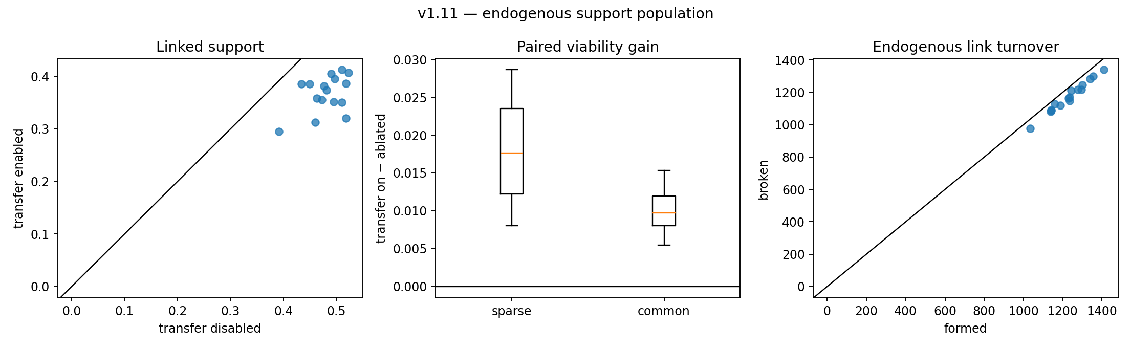
co_stabilization_population.py removes v1.10's supplied support graph. Individuals occupy a 12 × 12 toroidal lattice, receive environmental resources, suffer shocks, die, reproduce locally, and mutate. Support propensity and link propensity are inherited. Realized links form and break during the run; every link, transfer, self-repair, and birth is paid from stored energy. Low-contributing recipients are allowed, and there is no explicit fitness or group reward. The potential neighborhood remains spatially constrained, but the occupied population and realized support graph are endogenous.
The preregistered candidate criterion required three things: valid accounting, more linked support retained under transfer-enabled evolution than in a matched transfer-disabled control in a majority of seeds, and a positive paired sparse-shock assay after evolution. The first and third hold. The selection condition fails decisively.
| Median over 16 seeds | Transfers enabled | Transfers disabled |
|---|---|---|
| late population abundance | 104.1 | 125.6 |
| linked support propensity | 0.378 | 0.486 |
| realized link density | 0.485 | 0.489 |
- The network is dynamically produced. Median turnover is 1,236 links formed and 1,168 broken, with 96 births and 96 deaths. Maximum transfer draw / unused repair capacity is
1.000000; stored energy never becomes negative. - The network is functionally useful. In paired post-evolution sparse-pulse assays, enabling the exact evolved transfers adds
+0.0089survivors,+0.0176integrated viability, and a 2-step recovery advantage over ablating transfer. - But contribution is selected downward. Transfer-enabled populations retain less linked support in all 16 seeds: median difference
−0.1061, with a−0.1221change from the initial level. They also sustain fewer individuals. The support mechanism helps the present collective but costs its contributors enough that local survival and reproduction do not preserve it. - The common-mode boundary is partial. Common damage yields no median survivor gain and only
+0.0097integrated viability, below the sparse result; its recovery-time summary nevertheless improves by 3 rather than 2 steps. The limit is not universal across metrics. - Low contributors persist.
40.4%of linked agents finish below support0.20;17.6%combine that low contribution with link propensity above0.50.
The preregistered endogenous co-stabilization criterion is therefore not supported. v1.11 exposes the missing bridge between a mechanism that benefits a collective and one that evolution actually retains. The next discriminating models are not “more support” but mechanisms that can alter that selection problem: partner choice, conditional reciprocity, and spatial/kin assortment. Resource production and open-ended topology remain external beyond that.
v1.12 — visible contribution sorts the network but does not retain it (run)
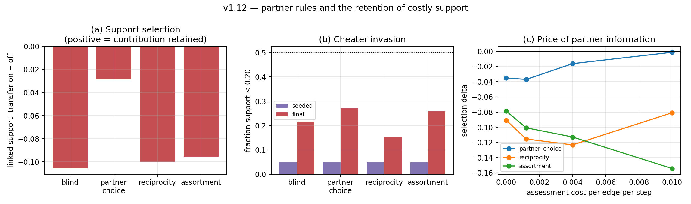
co_stabilization_selection.py takes up v1.11's diagnosis. In v1.11 a link forms with probability proportional to \(\sqrt{g_u g_v}\) over the link genes only; the support gene never enters, so a non-contributor is exactly as attractive a partner as a contributor. v1.12 asks whether making contribution visible to partner formation changes the selection outcome — and what that visibility costs.
Four arms share one accounting: blind (v1.11 unchanged), partner choice (both endpoints weight formation by the other's support, and links to low contributors break faster), conditional reciprocity (blind formation, but a donor scales its offer to each neighbour by decaying per-edge memory of what came back), and assortment (formation favours genetically similar partners). Following v1.10's matched-budget discipline, the three informed arms pay ASSESS_COST per assessed edge per step: free partner information would rig the comparison. The blind arm reproduces v1.11 trajectory-for-trajectory, so the arms differ only in the partner rule and its paid information.
| Median over 16 seeds | linked support on | off | delta | positive seeds | vs. start |
|---|---|---|---|---|---|
| blind | 0.375 | 0.483 | −0.1056 | 0% | −0.1277 |
| partner choice | 0.543 | 0.566 | −0.0287 | 19% | +0.0657 |
| reciprocity | 0.382 | 0.485 | −0.0999 | 0% | −0.0875 |
| assortment | 0.392 | 0.490 | −0.0956 | 0% | −0.0835 |
- The preregistered criterion is not supported. No arm reversed the sign of support selection in a majority of seeds. Partner choice weakens the loss by roughly a factor of four and is the only arm with any positive seeds, but 19% is not a majority.
- Partner choice protects the network, not the population. Seeded with 5% cheaters, the fraction of linked agents below support 0.20 ends at 1.2% versus 22.0% under blind — near-total exclusion. Yet the cheater fraction in the population as a whole still rises to 27.1%. Non-contributors are excluded rather than eliminated, and persist unlinked.
- One preregistered prediction did not apply. P4 expected a cost boundary: raise the price of partner information and the advantage should vanish. Instead partner choice's delta moves toward zero as cost rises (−0.0351 → −0.0012). A rewiring rule is not a taxed benefit; a higher price suppresses link formation in treatment and control alike. The prediction was the wrong shape for this mechanism, not a failed test of it.
- The measurement question is now itself open. Against the starting level rather than the matched control, partner choice is the only arm that does not decay (+0.0657). Where a rule rewards support even with transfer off, the control rises too, so the on/off delta understates absolute retention. Reported as a post-hoc diagnostic; the preregistered comparison stands as the verdict.
- The common-mode limit holds in every arm, as in v1.10 and v1.11.
Making contribution visible is therefore not sufficient to make it evolutionarily retainable in this model. It is enough to sort the network: costly support survives where partners can refuse, while non-contributors accumulate outside it. Whether an excluded population is a stable outcome or a reservoir waiting for the network to weaken is the next discriminating question.
v1.13 — relocating the cost nearly removes the penalty, and reverses invasion (run)
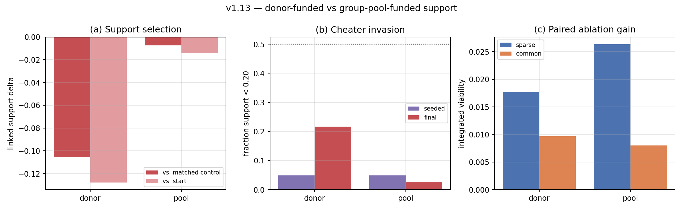
co_stabilization_pool.py tests the arm Log 019 preregistered. In v1.11 and v1.12 the cost of support falls entirely on the individual donor (support_i × spare_i). If who pays is the obstruction, moving the cost to the local group should retain the trait; if it is still selected down, the obstruction lies below the accounting, in the selection level itself.
Two arms, one accounting. donor is v1.11 unchanged. pool lets each connected component of the link graph fund support at a rate set by the group's mean support gene: every member pays that same rate on its own spare capacity regardless of its own gene, and damaged members draw by need. An individual's cost is thereby decoupled from its own generosity. This is "charge the veto to the institution, not the reviewer" made mechanical. The donor arm reproduces v1.11 trajectory-for-trajectory, which a test asserts, so the arms differ only in who bears the cost.
| Median over 16 seeds | linked support on | off | delta | positive seeds | vs. start | abundance | group size |
|---|---|---|---|---|---|---|---|
| donor | 0.375 | 0.483 | −0.1056 | 0% | −0.1277 | 104.5 | 7.7 |
| pool | 0.461 | 0.483 | −0.0075 | 44% | −0.0143 | 77.8 | 4.4 |
- The criterion is not met, but the penalty nearly vanishes. Selection against support drops from −0.1056 to −0.0075, and drift from the starting level from −0.1277 to −0.0143. Positive seeds rise from 0% to 44% — short of the majority the preregistration required.
- A preregistered prediction was falsified in the opposite direction. P3 predicted that pooling makes free-riding easier, since a mutant could pay the group rate while contributing nothing to it. The reverse happened: seeded with 4.9% cheaters, the donor arm ends at 21.6% while the pool arm ends at 2.6% — below its seeded level — with mean support 0.874 versus 0.713. Because the levy tracks the group mean, a low-support mutant inside a cooperative group cannot avoid paying, so defection buys it nothing. Relocation does not only dilute the penalty for contributing; it removes the reward for defecting.
- Relocation is not free. The pool arm sustains a smaller population (77.8 versus 104.5) and smaller groups (4.4 versus 7.7). The group pays in size for what it buys in retention.
- The common-mode limit holds and the low-support fraction among linked agents halves (20.2% versus 40.4%).
The honest reading is that this is the most informative of the four co-stabilization arms and still not a positive result. Two questions the model cannot settle: whether 44% would cross a majority under a longer horizon or weaker mutation, and — more importantly — whether what is seen here is selection for support or merely the absence of selection against it. With the levy set by the group mean, within-group variation in the gene is nearly cost-neutral, so drift rather than advantage may be carrying it. Distinguishing those two is the next discriminating measurement, not a larger version of this one.
Running
python inverse_benchmark.py              # v0: console summary, three testbeds (~10 s)
python inverse_benchmark.py --save       # also write the v0 figure (to lab/tools/)
python intervention_experiment.py        # v1.1: interventions vs. observation (~5 s)
python intervention_experiment.py --save # also write the intervention figure
python family_search.py                  # v1.2: the family-search wall (~1 s)
python family_search.py --save           # also write the family-search figure
python model_exploitation.py             # v1.3: exploitation vs class size (~2 min)
python model_exploitation.py --save      # also write the exploitation figure
python weakness_selector.py              # v1.4: weakness vs simplicity (~3 s)
python weakness_selector.py --save       # also write the weakness figure
python wmax_planner.py                   # v1.5: marking the guesses (~40 s)
python wmax_planner.py --save            # also write the wmax-planner figure
python closed_loop.py                    # v1.6: the closed loop (~30 s)
python closed_loop.py --save             # also write the closed-loop figure
python ensemble_size.py                  # v1.7: ensemble size vs the curse (~9 s)
python ensemble_size.py --save           # also write the ensemble figure
python composition.py                    # v1.8: composition, the empty class (~15 s)
python composition.py --save             # also write the composition figure
python co_stabilization.py               # v1.9: co-stabilization, the knockout (~5 s)
python co_stabilization.py --save        # also write the co-stabilization figure
python co_stabilization_redundancy.py      # v1.10: matched-budget redundancy (~25 s)
python co_stabilization_redundancy.py --save # also write the redundancy figure
python co_stabilization_population.py      # v1.11: endogenous population (~7 s)
python co_stabilization_population.py --save # also write the population figure
python co_stabilization_selection.py       # v1.12: partner rules, four arms (~80 s)
python co_stabilization_selection.py --save # also write the selection figure
python co_stabilization_pool.py            # v1.13: donor vs group-pool funding (~20 s)
python co_stabilization_pool.py --save     # also write the pool figure
Requires numpy, matplotlib only (repo requirements.txt).
Design note (2026-08-19). The v1.2–v1.7 suites index their experimental
settings — coverage masks, guesses, start rows, candidate draws — by dedicated
setting counters and run every setting against every rule; standard errors
are taken across settings. Previously each rule drew its own settings from its
position in the iteration order, which keys the draws to the target's loop
coordinate — the same error class as the recursive-workbench's fixed RNG leak,
one level up. The crossing changed no direction except one: v1.6's
anti-exploration corollary did not survive it and is withdrawn in place. Two
uniform-world results (v1.2's elegance-is-chance, v1.4's
committing-buys-nothing) became identities. Headline claims are guarded by
tests/test_benchmark_v1_headlines.py at small declared crossed grids.
Current roadmap (open)
(The benchmark sequence through v1.13 is run and documented above. The items below remain open.)
- Is it selection or only the absence of selection?: v1.13 moved the cost of support from the donor to the local group. Selection against the trait nearly vanished (−0.0075 versus −0.1056) and seeded cheaters fell below their starting frequency (2.6% versus 21.6%), but positive seeds reached only 44% and population size dropped. Because a group-mean levy makes within-group variation nearly cost-neutral, the retained support may be drift rather than advantage. The next arm must separate those: a within-group cost gradient that keeps relocation while restoring a measurable selection differential, plus longer horizons and weaker mutation to test whether 44% is a boundary or a plateau. Endogenous resource production and open topology remain beyond that.
- Learned searchers vs. the enumerator: family_search.py measures one exhaustive search. Compare learned and symbolic searchers on the same DSL, targets, compute budget, and held-out interventions rather than assuming either has a generic advantage.
- Re-simulation divergence as a behavioral metric: does a recovered candidate process model match held-out trajectories and interventions even when its parameters differ?
- IFS testbed: recover contractive affine maps from an attractor point cloud (hard even with known family — no time ordering).
- Cross-method comparison: hand-rolled least squares (v0) vs. SINDy/PySR as external baselines (would add dependencies; deliberately out of v0).
Related
- The Generator Question — the superseded spine that motivated the benchmark; retained as audit history.
- Measurement as Weak Intervention — the conceptual hinge on v1.1's hierarchy: coupling is not identification; plus the fourth (reflexive) regime the toys cannot exhibit.
- Open Problems — Open Problem 11 (bounded inverse reconstruction).
- Related Work Map — SINDy / system identification / program induction anchors.
lab/experiments/trace_to_generator/— the earlier inverse-prompting scaffold.trace-to-generator-small— a compact learned sequence model trained from scratch on controlled synthetic traces; implementation ready, no research run yet.